Chapter 2
2.1 A Preview of Calculus
Learning Objectives
By the end of this section, you should be able to:
- Describe the tangent problem and how it led to the idea of the derivative.
- Explain how the idea of a limit is involved in solving the tangent problem.
- Recognize the tangent line to a curve at a point as the limit of secant lines.
- Identify instantaneous velocity as the limit of average velocity over a shrinking time interval.
- Describe the area problem and how it is solved by the integral.
- Explain how the idea of a limit is involved in solving the area problem.
- Recognize how limits, derivatives, and integrals lead naturally to the study of infinite series and multivariable calculus.
Calculus grew out of practical problems that classical algebra and geometry could not crack on their own. Two questions led to its creation:
- The tangent problem — how do we measure the slope of a curve at a single point?
- The area problem — how do we measure the area trapped between a curve and the x-axis?
Both questions have the same secret ingredient: a limit. The rest of this chapter — and most of single-variable calculus — is the story of how that one idea unlocks both.
2.1.1 The Tangent Problem and Differential Calculus
The secant line to the function \(f(x)\) through the points \((a, f(a))\) and \((x, f(x))\) is the line passing through these two points. Its slope is
$$m_{\sec} = \frac{f(x) - f(a)}{x - a} \qquad \text{(Equation 2.1)}$$We don't have the tools yet to measure the slope AT a single point on a curve — slope needs two points to compute (rise over run). The secant is a workaround: it uses two points we can work with, then we squeeze them together until they're almost the same point. The slope of that almost-the-same-point line is what we'll call the slope at \(a\).
Rate of change is one of the most critical ideas in calculus. Linear functions have a single, constant slope — that slope IS the rate of change everywhere. Figure 2.2 shows three lines and the constant slopes they encode: \(f(x) = -2x - 3\) drops by 2 for every unit right, \(g(x) = \tfrac{1}{2}x + 1\) climbs by \(\tfrac{1}{2}\), and \(h(x) = 2\) never changes.
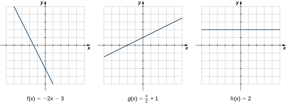
Figure 2.2 — The rate of change of a linear function is constant in each of these three graphs, with the constant determined by the slope.
Now compare those lines to \(k(x) = x^2\) (Figure 2.3). This curve falls steeply on the left, levels off near the bottom, and climbs back up — increasingly fast — on the right. There is no single slope. The rate of change at \(x = -2\) is wildly different from the rate at \(x = 2\). So we have to ask: how do we measure the rate of change of a function whose slope keeps changing?
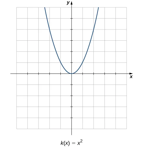
Figure 2.3 — The function \(k(x) = x^2\) does not have a constant rate of change.
The trick is to start by approximating with a secant line — exactly the construction Definition 2.1.1 names. Figure 2.4 shows a single secant through \((a, f(a))\) and a nearby point \((x, f(x))\); its slope estimates how steep the curve is at \(a\).
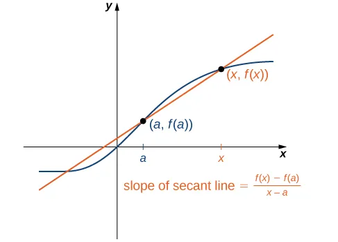
Figure 2.4 — The slope of a secant line through a point \((a, f(a))\) estimates the rate of change of the function at the point \((a, f(a))\).
How good is the secant-line estimate? It depends on how close \(x\) is to \(a\). The closer they are, the better the secant slope mimics the actual rate of change of \(f(x)\) at \(a\). Figure 2.5 shows three secants getting tighter and tighter on the same target point.
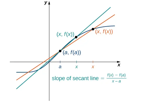
Figure 2.5 — As \(x\) gets closer to \(a\), the slope of the secant line becomes a better approximation to the rate of change of the function \(f(x)\) at \(a\).
As we slide \(x\) toward \(a\), the secant lines themselves approach a single line — the tangent line to \(f(x)\) at \(a\) (Figure 2.6). The slope of that tangent line is the true rate of change of the function at \(a\). It also has another name: the derivative of \(f\) at \(a\), written \(f'(a)\). Differential calculus is the branch of calculus that studies derivatives and what they can tell us.
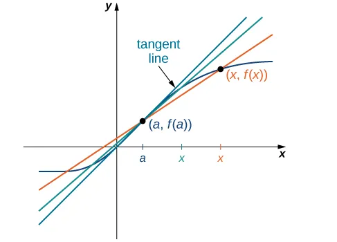
Figure 2.6 — Solving the Tangent Problem: As \(x\) approaches \(a\), the secant lines approach the tangent line.
Example 2.1.1 puts the formula to work. We'll estimate the slope of the tangent to \(f(x) = x^2\) at \(x = 1\) by computing secant slopes through nearby points.
Let \(s(t)\) be the position of an object moving along a coordinate axis at time \(t\). The average velocity of the object over a time interval \([a, t]\) (where \(a < t\), or \([t, a]\) if \(t < a\)) is
$$v_{\text{ave}} = \frac{s(t) - s(a)}{t - a} \qquad \text{(Equation 2.2)}$$Notice that Equation 2.2 has the same shape as Equation 2.1 — change in output over change in input. Average velocity is literally the slope of the secant line on a position-vs-time graph. As we choose \(t\) closer and closer to \(a\), that average velocity tightens toward the instantaneous velocity at \(t = a\) — the slope of the tangent line on the position graph. The squeeze process is exactly the same as before, and it has a name.
For a position function \(s(t)\), the instantaneous velocity at a time \(t = a\) is the value that the average velocities approach on intervals of the form \([a, t]\) or \([t, a]\) as the values of \(t\) become closer to \(a\), provided such a value exists.
This squeeze process — letting \(x\) approach \(a\), or \(t\) approach \(a\), inside an expression like a slope or an average — is called taking a limit. It's the central idea of single-variable calculus. Definitions 2.1.1, 2.1.2, and 2.1.3 all set the stage; Chapter 2's later sections make limits formal.
Example 2.1.2 shows the squeeze in action: two short intervals on either side of \(t = 0.5\) give two average velocities that bracket the instantaneous value.
Estimate the slope of the tangent line (rate of change) to \(f(x) = x^2\) at \(x = 1\) by finding the slope of the secant line through \((1, 1)\) and the point \(\left(\tfrac{5}{4}, \tfrac{25}{16}\right)\) on the graph of \(f(x) = x^2\).
Solution
Apply Equation 2.1 with \(a = 1\), \(f(a) = 1\), \(x = \tfrac{5}{4}\), \(f(x) = \tfrac{25}{16}\):
$$m_{\sec} = \frac{\tfrac{25}{16} - 1}{\tfrac{5}{4} - 1} = \frac{\tfrac{9}{16}}{\tfrac{1}{4}} = \frac{9}{16} \cdot \frac{4}{1} = \frac{9}{4} = 2.25.$$Answer: The secant slope is \(2.25\). Since \(\tfrac{5}{4}\) is closer to \(1\) than the points in Example 2.1.1, this is our best estimate yet — the tangent slope at \(x = 1\) is somewhere close to \(2.25\) (and in fact equals exactly \(2\), as we will confirm later in the chapter).
The same "shrink toward a single point" idea applies to motion. Velocity is the rate of change of position, so we can ask: if \(s(t)\) gives the position of an object at time \(t\), what is the object's velocity at one specific instant \(t = a\)? Just like with secant slopes, we start by averaging over a short interval.
Recall from algebra: the speed of an object moving at a constant rate equals distance traveled divided by time elapsed. We extend that idea to a changing-position function by defining average velocity over a time interval to be the change in position divided by the length of the interval.
Estimate the slope of the tangent line (rate of change) to \(f(x) = x^2\) at \(x = 1\) by finding slopes of secant lines through \((1, 1)\) and each of the following points on the graph of \(f(x) = x^2\):
a) \((2, 4)\)
b) \(\left(\tfrac{3}{2}, \tfrac{9}{4}\right)\)
Solution
Apply Equation 2.1 with \(a = 1\) and \(f(a) = 1\).
Step 1 — Secant through \((1, 1)\) and \((2, 4)\):
$$m_{\sec} = \frac{4 - 1}{2 - 1} = \frac{3}{1} = 3.$$Step 2 — Secant through \((1, 1)\) and \(\left(\tfrac{3}{2}, \tfrac{9}{4}\right)\):
$$m_{\sec} = \frac{\tfrac{9}{4} - 1}{\tfrac{3}{2} - 1} = \frac{\tfrac{5}{4}}{\tfrac{1}{2}} = \frac{5}{2} = 2.5.$$Step 3 — Compare and estimate:
The second point sits much closer to \((1, 1)\), so the slope \(2.5\) is the better estimate of the tangent slope. The true tangent slope is somewhere in the band between \(2\) and \(2.5\) — and a tighter second point would give an even sharper estimate.
Answer: A reasonable estimate for the slope of the tangent line at \((1, 1)\) is roughly \(2\) to \(2.5\) (Figure 2.7).
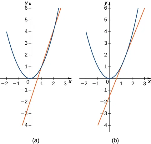
Figure 2.7 — The secant lines to \(f(x) = x^2\) at \((1, 1)\) through (a) \((2, 4)\) and (b) \(\left(\tfrac{3}{2}, \tfrac{9}{4}\right)\) provide successively closer approximations to the tangent line to \(f(x) = x^2\) at \((1, 1)\).
An object moves along a coordinate axis so that its position at time \(t\) is given by \(s(t) = t^3\). Estimate its instantaneous velocity at time \(t = 2\) by computing its average velocity over the time interval \([2, 2.001]\).
Solution
Apply Equation 2.2 with \(a = 2\) and \(t = 2.001\).
Step 1 — Compute \(s(2)\) and \(s(2.001)\):
$$s(2) = 2^3 = 8,$$ $$s(2.001) = (2.001)^3 = 8.012006001.$$Step 2 — Average velocity:
$$v_{\text{ave}} = \frac{s(2.001) - s(2)}{2.001 - 2} = \frac{8.012006001 - 8}{0.001} = \frac{0.012006001}{0.001} = 12.006001.$$Answer: \(v_{\text{ave}} \approx 12.006\). Because the interval is very short, this average is an excellent estimate of the instantaneous velocity at \(t = 2\): \(v(2) \approx 12\).
A rock is dropped from a height of \(64\) feet. Its height above the ground (in feet) \(t\) seconds later (for \(0 \le t \le 2\)) is given by \(s(t) = -16t^2 + 64\). Find the average velocity of the rock over each of these time intervals, and use the results to guess the instantaneous velocity at \(t = 0.5\):
a) \([0.49, 0.5]\)
b) \([0.5, 0.51]\)
Solution
Apply Equation 2.2.
Step 1 — Compute \(s\) at the four endpoints:
$$s(0.49) = -16(0.49)^2 + 64 = 64 - 3.8416 = 60.1584,$$ $$s(0.5) = -16(0.5)^2 + 64 = 64 - 4 = 60,$$ $$s(0.51) = -16(0.51)^2 + 64 = 64 - 4.1616 = 59.8384.$$Step 2 — Average velocity over \([0.49, 0.5]\):
$$v_{\text{ave}} = \frac{s(0.5) - s(0.49)}{0.5 - 0.49} = \frac{60 - 60.1584}{0.01} = \frac{-0.1584}{0.01} = -15.84 \text{ ft/sec}.$$Step 3 — Average velocity over \([0.5, 0.51]\):
$$v_{\text{ave}} = \frac{s(0.51) - s(0.5)}{0.51 - 0.5} = \frac{59.8384 - 60}{0.01} = \frac{-0.1616}{0.01} = -16.16 \text{ ft/sec}.$$Step 4 — Estimate the instantaneous velocity:
The two average velocities bracket the instantaneous value: \(-15.84\) and \(-16.16\). The instantaneous velocity at \(t = 0.5\) must sit between them.
Answer: Best guess: \(v(0.5) \approx -16\) ft/sec. (The negative sign means the rock is falling — height is decreasing.)
2.1.2 The Area Problem and Integral Calculus
The second great question that gave birth to calculus is about area. Many physical quantities — work done by a force, distance traveled when speed is changing, electrical charge, probability — can be read off as an area trapped under a curve. So we ask: how do we find the area between the graph of a function and the x-axis over an interval (Figure 2.8)?
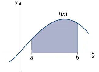
Figure 2.8 — The Area Problem: How do we find the area of the shaded region?
The plan looks familiar: start by approximating. Slice the interval \([a, b]\) into thin pieces and stand a rectangle on each piece, with the height set by the function's value somewhere in that slice. Add up the rectangle areas. That sum is a rough estimate of the area under the curve (Figure 2.9).
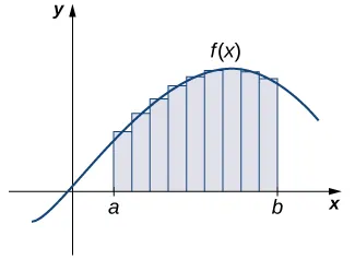
Figure 2.9 — The area of the region under the curve is approximated by summing the areas of thin rectangles.
As we slice thinner and thinner — width approaching zero — the rectangle-sum approaches the true area between the curve and the x-axis over \([a, b]\). It is, once again, a limit. The number that the sums approach is called the definite integral of \(f\) on \([a, b]\), and integral calculus is the branch of calculus built around it.
Estimate the area between the x-axis and the graph of \(f(x) = x^2 + 1\) over the interval \([0, 3]\) by using the three rectangles shown in the figure below.
![Three right-endpoint rectangles over [0,3] under f(x) = x<sup>2</sup> + 1 (alternate to Figure 2.10).](../images/figure_ex_2.1.10.png)
Solution
This alternate figure shades rectangles using the RIGHT endpoint of each unit-width slice as the height. The heights become \(f(1) = 2\), \(f(2) = 5\), and \(f(3) = 10\).
Step 1 — Add the right-endpoint rectangle areas:
$$\text{Estimated area} = 1 \cdot 2 + 1 \cdot 5 + 1 \cdot 10 = 17 \text{ unit}^2.$$Answer: \(17\) square units. This time the estimate OVERSHOOTS the true area of \(12\) square units — because each rectangle uses the height at the RIGHT edge, where the curve is higher. Notice the true answer (\(12\)) sits neatly between the left-endpoint estimate (\(8\), from Example 2.1.3) and this right-endpoint estimate (\(17\)). Taking thinner rectangles closes the gap from both sides.
Estimate the area between the x-axis and the graph of \(f(x) = x^2 + 1\) over the interval \([0, 3]\) by using the three rectangles shown in Figure 2.10.
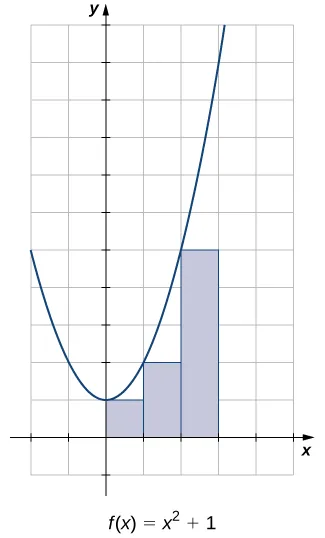
Figure 2.10 — The area of the region under the curve of \(f(x) = x^2 + 1\) can be estimated using rectangles.
Solution
Step 1 — Read each rectangle's area from the figure:
The three rectangles in Figure 2.10 have heights set by the left endpoint of each unit-width slice: \(f(0) = 1\), \(f(1) = 2\), and \(f(2) = 5\). Each rectangle has width \(1\), so the areas are \(1 \cdot 1 = 1\) square unit, \(1 \cdot 2 = 2\) square units, and \(1 \cdot 5 = 5\) square units.
Step 2 — Sum the areas:
$$\text{Estimated area} = 1 + 2 + 5 = 8 \text{ unit}^2.$$Answer: The estimate is \(8\) square units. The true area under \(f(x) = x^2 + 1\) on \([0, 3]\) is \(12\) square units — the rectangle estimate undershoots because each rectangle uses the height at the LEFT edge of its slice (where the curve is lower).
2.1.3 Other Aspects of Calculus
So far we have only studied functions of one variable, where the graph lives in two dimensions. There is no reason to stop there. What if instead of an object moving along a coordinate axis, we want the velocity of a rock fired from a catapult, or of an airplane moving in three dimensions? What if we want to compute volumes of solid shapes — like the surface shown in Figure 2.11? These questions live in multivariable calculus, the branch of the subject that studies functions of two or more variables.
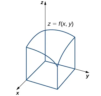
Figure 2.11 — We can use multivariable calculus to find the volume between a surface defined by a function of two variables and a plane.
Before we can climb to multivariable calculus, though, we have to build the single-variable foundation. That starts with the concept this section has gestured at over and over: the limit. The rest of Chapter 2 makes limits precise.
Problem Set 2.1
Using the definition, determine whether the function
$$ f(x)=\begin{cases}2x+1 & \text{if } x<1 \\ 2 & \text{if } x=1 \\ -x+4 & \text{if } x>1\end{cases} $$is continuous at \(x=1\). If the function is not continuous at 1, indicate which condition for continuity at a point fails to hold.
Solution
Step 1 — Condition (i): \(f(1)=2\), so the point is defined.
Step 2 — Condition (ii): Compute one-sided limits.
$$ \lim_{x\to 1^-}f(x)=2(1)+1=3, \qquad \lim_{x\to 1^+}f(x)=-(1)+4=3. $$Both one-sided limits equal 3, so \(\lim_{x\to 1}f(x)=3\). Condition (ii) holds.
Step 3 — Condition (iii): Compare. \(f(1)=2\) but \(\lim_{x\to 1}f(x)=3\). The values disagree, so condition (iii) fails.
Answer: \(f\) is discontinuous at \(x=1\); condition (iii) fails.
Using the definition, determine whether the function \(f(x)=\dfrac{x^2-4}{x-2}\) is continuous at \(x=2\). Justify the conclusion.
Solution
Step 1 — Test condition (i). Try to evaluate \(f(2)\):
$$ f(2)=\frac{2^2-4}{2-2}=\frac{0}{0}, $$which is undefined. Condition (i) fails immediately.
Step 2 — Stop. Once condition (i) fails, we don't need to test conditions (ii) and (iii) to conclude discontinuity. The function \(f(x)=\dfrac{x^2-4}{x-2}\) is discontinuous at \(x=2\) because \(f(2)\) is undefined. The graph of \(f(x)\) is shown in Figure 2.35.
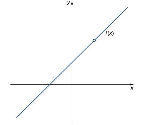
Figure 2.35 — The function \(f(x)\) is discontinuous at 2 because \(f(2)\) is undefined.
Answer: Discontinuous at \(x=2\); condition (i) fails.
For what values of \(x\) is \(f(x)=3x^4-4x^2\) continuous?
Solution
Step 1 — Identify the function type. This is a polynomial — only sums, products, and integer powers of \(x\) and constants.
Step 2 — Apply the theorem. Polynomials are continuous on their entire domain, which is all real numbers.
Answer: Continuous on \((-\infty,\infty)\) — every real number.
Using the definition, determine whether the function
$$ f(x)=\begin{cases}-x^2+4 & \text{if } x\le 3 \\ 4x-8 & \text{if } x>3\end{cases} $$is continuous at \(x=3\). Justify the conclusion.
Solution
Step 1 — Test condition (i). Because \(x=3\) lies on the \(x\le 3\) branch, use the top formula:
$$ f(3)=-(3)^2+4=-5. $$So \(f(3)\) is defined. Condition (i) holds.
Step 2 — Test condition (ii). Compute the two one-sided limits. From the left we are still on the top branch:
$$ \lim_{x\to 3^-}f(x)=-(3)^2+4=-5. $$From the right we switch to the bottom branch:
$$ \lim_{x\to 3^+}f(x)=4(3)-8=4. $$The two one-sided limits disagree, so \(\lim_{x\to 3}f(x)\) does not exist. Condition (ii) fails.
Step 3 — Stop. The function is discontinuous at \(x=3\). The graph of \(f(x)\) is shown in Figure 2.36.
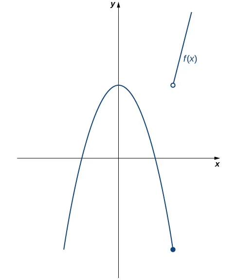
Figure 2.36 — The function \(f(x)\) is not continuous at 3 because \(\lim_{x\to 3}f(x)\) does not exist.
Answer: Discontinuous at \(x=3\); condition (ii) fails.
Using the definition, determine whether the function
$$ f(x)=\begin{cases}\dfrac{\sin x}{x} & \text{if } x\ne 0 \\ 1 & \text{if } x=0\end{cases} $$is continuous at \(x=0\).
Solution
Step 1 — Test condition (i). The piecewise branch at \(x=0\) gives \(f(0)=1\). Condition (i) holds.
Step 2 — Test condition (ii). From the previous section we know the famous trig limit:
$$ \lim_{x\to 0}f(x)=\lim_{x\to 0}\frac{\sin x}{x}=1. $$Condition (ii) holds.
Step 3 — Test condition (iii). Compare:
$$ f(0)=1=\lim_{x\to 0}f(x). $$Condition (iii) holds. All three conditions are satisfied.
Answer: \(f(x)\) is continuous at \(x=0\).
For what values of \(x\) is \(f(x)=\dfrac{x+1}{x-5}\) continuous?
Solution
Step 1 — Identify the domain. This is a rational function, so it is defined wherever the denominator is nonzero. \(x-5=0\) when \(x=5\), so the domain is every real number except \(5\).
Step 2 — Apply the theorem. Rational functions are continuous on their domains, so \(f(x)\) is continuous for every real \(x\) except \(x=5\).
Answer: Continuous on \((-\infty,5)\cup(5,\infty)\).
For
$$ f(x)=\begin{cases}x^2 & \text{if } x\ne 1 \\ 3 & \text{if } x=1\end{cases}, $$decide whether \(f\) is continuous at \(1\). If \(f\) is not continuous at \(1\), classify the discontinuity as removable, jump, or infinite.
Solution
Step 1 — Check continuity. \(f(1)=3\) (defined). The limit comes from the \(x\ne 1\) branch, so
$$ \lim_{x\to 1}f(x)=\lim_{x\to 1}x^2=1. $$Since \(f(1)=3\ne 1=\lim_{x\to 1}f(x)\), condition (iii) fails — discontinuous at 1.
Step 2 — Classify. The two-sided limit exists (as the real number 1), so by Definition 2.2(1) this is a removable discontinuity.
Answer: Removable discontinuity at \(x=1\); redefining \(f(1)=1\) would restore continuity.
In Example 2.4.1, we showed that \(f(x)=\dfrac{x^2-4}{x-2}\) is discontinuous at \(x=2\). Classify this discontinuity as removable, jump, or infinite.
Solution
Step 1 — Compute the limit. Factor the top and cancel:
$$ \begin{aligned} \lim_{x\to 2}f(x) &=\lim_{x\to 2}\frac{x^2-4}{x-2} \\ &=\lim_{x\to 2}\frac{(x-2)(x+2)}{x-2} \\ &=\lim_{x\to 2}(x+2) \\ &=4. \end{aligned} $$Step 2 — Read the label. The limit exists (as the real number 4), so by Definition 2.2(1) the discontinuity is removable.
Answer: Removable discontinuity at \(x=2\). If we redefined \(f(2)=4\), continuity would be restored.
In Example 2.4.2 we showed that
$$ f(x)=\begin{cases}-x^2+4 & \text{if } x\le 3 \\ 4x-8 & \text{if } x>3\end{cases} $$is discontinuous at \(x=3\). Classify this discontinuity as removable, jump, or infinite.
Solution
Step 1 — Recall the one-sided limits. From Example 2.4.2,
$$ \lim_{x\to 3^-}f(x)=-5 \qquad \text{and} \qquad \lim_{x\to 3^+}f(x)=4. $$Step 2 — Read the label. Both one-sided limits exist (real numbers, not \(\pm\infty\)) but they disagree. By Definition 2.2(2), the discontinuity is a jump.
Answer: Jump discontinuity at \(x=3\).
Determine whether \(f(x)=\dfrac{x+2}{x+1}\) is continuous at \(-1\). If the function is discontinuous at \(-1\), classify the discontinuity as removable, jump, or infinite.
Solution
Step 1 — Check the function value. \(f(-1)\) requires dividing by \(-1+1=0\), which is undefined. So \(f\) is discontinuous at \(-1\).
Step 2 — Compute one-sided limits. As \(x\to -1\), the numerator approaches \(1\) and the denominator approaches \(0\). The sign of the denominator decides which infinity:
$$ \lim_{x\to -1^-}\frac{x+2}{x+1}=-\infty, \qquad \lim_{x\to -1^+}\frac{x+2}{x+1}=+\infty. $$Step 3 — Read the label. At least one (in fact both) one-sided limits are infinite, so by Definition 2.2(3), the discontinuity is infinite.
Answer: Infinite discontinuity at \(x=-1\) — there is a vertical asymptote there.
State the interval(s) over which the function \(f(x)=\sqrt{x+3}\) is continuous.
Solution
Step 1 — Find the domain. \(x+3\ge 0\) gives \(x\ge -3\), so the domain is \([-3,\infty)\).
Step 2 — Check the open interior. For every \(a>-3\), the root law gives \(\lim_{x\to a}\sqrt{x+3}=\sqrt{a+3}=f(a)\), so \(f\) is continuous on \((-3,\infty)\).
Step 3 — Check the left endpoint. \(\lim_{x\to -3^+}\sqrt{x+3}=0=f(-3)\), so \(f\) is continuous from the right at \(-3\).
Answer: Continuous over \([-3,\infty)\).
State the interval(s) over which the function \(f(x)=\dfrac{x-1}{x^2+2x}\) is continuous.
Solution
Step 1 — Find the domain. The denominator factors as \(x(x+2)\) and equals zero when \(x=0\) or \(x=-2\). So the domain is every real number except those two values:
$$ (-\infty,-2)\cup(-2,0)\cup(0,+\infty). $$Step 2 — Apply the rational-function theorem. Rational functions are continuous everywhere on their domain. So \(f(x)\) is continuous on each of the three intervals above.
Answer: Continuous over \((-\infty,-2)\), \((-2,0)\), and \((0,+\infty)\).
Evaluate \(\displaystyle\lim_{x\to \pi}\sin(x-\pi).\)
Solution
Step 1 — Identify the composition. Outer: \(\sin x\) (continuous at \(0\)). Inner: \(g(x)=x-\pi\).
Step 2 — Inner limit. \(\displaystyle\lim_{x\to \pi}(x-\pi)=0\).
Step 3 — Push the limit through.
$$ \lim_{x\to \pi}\sin(x-\pi)=\sin\!\left(\lim_{x\to \pi}(x-\pi)\right)=\sin(0)=0. $$Answer: \(0\).
State the interval(s) over which the function \(f(x)=\sqrt{4-x^2}\) is continuous.
Solution
Step 1 — Find the domain. We need \(4-x^2\ge 0\), i.e. \(-2\le x\le 2\). So the domain is the closed interval \([-2,2]\).
Step 2 — Check continuity on the open interior. From the limit laws (root law), for every \(a\in(-2,2)\):
$$ \lim_{x\to a}\sqrt{4-x^2}=\sqrt{4-a^2}=f(a), $$so \(f\) is continuous at every interior point.
Step 3 — Check the endpoints. At \(x=-2\), only the right-hand limit makes sense (the domain doesn't extend to the left). Compute:
$$ \lim_{x\to -2^+}\sqrt{4-x^2}=\sqrt{4-4}=0=f(-2), $$so \(f\) is continuous from the right at \(-2\). Symmetrically at \(x=2\):
$$ \lim_{x\to 2^-}\sqrt{4-x^2}=0=f(2), $$so \(f\) is continuous from the left at \(2\).
Step 4 — Combine. \(f\) is continuous over \([-2,2]\).
Answer: Continuous over \([-2,2]\).
Evaluate \(\displaystyle\lim_{x\to \pi/2}\cos\!\left(x-\dfrac{\pi}{2}\right).\)
Solution
Step 1 — Spot the composition. The function is \(\cos\bigl(g(x)\bigr)\) where \(g(x)=x-\dfrac{\pi}{2}\) is the inner function.
Step 2 — Compute the inner limit.
$$ \lim_{x\to \pi/2}\!\left(x-\frac{\pi}{2}\right)=\frac{\pi}{2}-\frac{\pi}{2}=0. $$Step 3 — Push the limit through. Because \(\cos x\) is continuous at \(0\), the composite function theorem applies:
$$ \lim_{x\to \pi/2}\cos\!\left(x-\frac{\pi}{2}\right)=\cos\!\left(\lim_{x\to \pi/2}\!\left(x-\frac{\pi}{2}\right)\right)=\cos(0)=1. $$Answer: \(1\).
Show that \(f(x)=x^3-x^2-3x+1\) has a zero over the interval \([0,1]\).
Solution
Step 1 — Check continuity. Polynomials are continuous on \((-\infty,\infty)\), so \(f\) is continuous on \([0,1]\). IVT applies.
Step 2 — Evaluate endpoints.
$$ f(0)=0-0-0+1=1>0, \qquad f(1)=1-1-3+1=-2<0. $$Step 3 — Apply the IVT with \(z=0\). Since \(0\) lies between \(-2\) and \(1\), there exists a \(c\) in \([0,1]\) with \(f(c)=0\).
Answer: \(f(x)=x^3-x^2-3x+1\) has at least one zero in \([0,1]\).
Show that \(f(x)=x-\cos x\) has at least one zero.
Solution
Step 1 — Check continuity. \(f(x)=x-\cos x\) is a difference of two functions that are continuous on \((-\infty,+\infty)\), so \(f\) itself is continuous everywhere. The IVT will apply on any closed interval.
Step 2 — Find an interval with sign change. Try the endpoints \(a=0\) and \(b=\pi/2\):
$$ f(0)=0-\cos(0)=-1<0, $$ $$ f\!\left(\frac{\pi}{2}\right)=\frac{\pi}{2}-\cos\!\left(\frac{\pi}{2}\right)=\frac{\pi}{2}-0=\frac{\pi}{2}>0. $$Step 3 — Apply the IVT with \(z=0\). Since \(f\) is continuous on \([0,\pi/2]\) and \(0\) lies between \(f(0)=-1\) and \(f(\pi/2)=\pi/2\), the IVT guarantees a number \(c\) in \([0,\pi/2]\) with \(f(c)=0\).
Answer: \(f(x)=x-\cos x\) has at least one zero in the interval \([0,\pi/2]\).
If \(f(x)\) is continuous over \([0,2]\), \(f(0)>0\), and \(f(2)>0\), can we use the Intermediate Value Theorem to conclude that \(f(x)\) has no zeros in the interval \([0,2]\)? Explain.
Solution
Step 1 — Read the theorem carefully. The IVT only guarantees the existence of a value \(c\) where \(f(c)=z\) when \(z\) lies between \(f(a)\) and \(f(b)\). When both endpoints are positive, the IVT says nothing about values that are not between them — like \(z=0\).
Step 2 — Counterexample. Consider \(f(x)=(x-1)^2\). It is continuous on \([0,2]\) with \(f(0)=1>0\) and \(f(2)=1>0\), yet \(f(1)=0\). So the function has a zero even though both endpoint values are positive.
Answer: No. The IVT does not say the function cannot reach values outside the bracket \([f(a),f(b)]\); it only guarantees it does reach the values inside.
For \(f(x)=\dfrac{1}{x}\), \(f(-1)=-1<0\) and \(f(1)=1>0\). Can we conclude that \(f(x)\) has a zero in the interval \([-1,1]\)?
Solution
Step 1 — Check the IVT hypotheses. The IVT requires \(f\) to be continuous on the entire closed interval \([-1,1]\). But \(f(x)=\dfrac{1}{x}\) is undefined at \(x=0\), which is in \([-1,1]\). So \(f\) is not continuous on \([-1,1]\) — there's an infinite discontinuity at \(0\).
Step 2 — Conclusion. The hypotheses of the IVT are not satisfied, so the theorem does not apply. In fact, \(\dfrac{1}{x}\) is never zero — the sign flip across \(0\) happens because the function blows up to \(\pm\infty\), not because it crosses through zero.
Answer: No — the IVT requires continuity over the whole closed interval, and \(\dfrac{1}{x}\) is not continuous at \(0\).
For the following exercises, points \(P(1, 2)\) and \(Q(x, y)\) are on the graph of the function \(f(x) = x^2 + 1\).
Problem 1. [T] Complete the following table with the appropriate values: the \(y\)-coordinate of \(Q\), the point \(Q(x, y)\), and the slope of the secant line passing through points \(P\) and \(Q\). Round your answer to eight significant digits.
| \(x\) | \(y\) | \(Q(x, y)\) | \(m_{\sec}\) |
|---|---|---|---|
| \(1.1\) | a. | e. | i. |
| \(1.01\) | b. | f. | j. |
| \(1.001\) | c. | g. | k. |
| \(1.0001\) | d. | h. | l. |
Problem 2. Use the values in the right column of the table in the preceding exercise to guess the value of the slope of the line tangent to \(f\) at \(x = 1\).
Problem 3. Use the value in the preceding exercise to find an equation of the tangent line at point \(P\). Graph \(f(x)\) and the tangent line.
Solutions 1–3
Problem 1
Step 1 — Set up the secant slope formula: For each \(x\), compute \(y = f(x) = x^2 + 1\), form the point \(Q(x, y)\), and apply the secant slope formula \(m_{\sec} = \dfrac{y - 2}{x - 1}\). The expression simplifies algebraically to \(m_{\sec} = \dfrac{x^2 - 1}{x - 1} = x + 1\) for \(x \ne 1\), which gives a quick sanity check on each numerical row.
Step 2 — Compute each row:
| \(x\) | \(y\) | \(Q(x, y)\) | \(m_{\sec}\) |
|---|---|---|---|
| \(1.1\) | \(2.21\) | \((1.1,\ 2.21)\) | \(2.1000000\) |
| \(1.01\) | \(2.0201\) | \((1.01,\ 2.0201)\) | \(2.0100000\) |
| \(1.001\) | \(2.002001\) | \((1.001,\ 2.002001)\) | \(2.0010000\) |
| \(1.0001\) | \(2.00020001\) | \((1.0001,\ 2.00020001)\) | \(2.0001000\) |
Answer: Slopes column reads \(2.1\), \(2.01\), \(2.001\), \(2.0001\) — clearly trending toward \(2\).
Problem 2
Step 1 — Read the trend: The four secant slopes from the previous table are \(2.1\), \(2.01\), \(2.001\), \(2.0001\). Each is closer to \(2\) than the one above it.
Answer: The slope of the tangent line at \(x = 1\) is approximately \(\boxed{2}\).
Problem 3
Step 1 — Apply point-slope form: With slope \(m = 2\) at the point \(P(1, 2)\),
$$y - 2 = 2(x - 1).$$
Step 2 — Solve for \(y\):
$$y = 2x.$$
Answer: The tangent line at \(P(1, 2)\) is \(y = 2x\). To graph, plot the parabola \(f(x) = x^2 + 1\) and the line \(y = 2x\); they touch at \((1, 2)\) and the line lies tangent there (under the parabola elsewhere).
For the following exercises, points \(P(1, 1)\) and \(Q(x, y)\) are on the graph of the function \(f(x) = x^3\).
Problem 4. [T] Complete the following table with the appropriate values: the \(y\)-coordinate of \(Q\), the point \(Q(x, y)\), and the slope of the secant line passing through points \(P\) and \(Q\). Round your answer to eight significant digits.
| \(x\) | \(y\) | \(Q(x, y)\) | \(m_{\sec}\) |
|---|---|---|---|
| \(1.1\) | a. | e. | i. |
| \(1.01\) | b. | f. | j. |
| \(1.001\) | c. | g. | k. |
| \(1.0001\) | d. | h. | l. |
Problem 5. Use the values in the right column of the table in the preceding exercise to guess the value of the slope of the tangent line to \(f\) at \(x = 1\).
Problem 6. Use the value in the preceding exercise to find an equation of the tangent line at point \(P\). Graph \(f(x)\) and the tangent line.
Solutions 4–6
Problem 4
Step 1 — Set up the secant slope formula: For each \(x\), compute \(y = x^3\), form \(Q(x, y)\), and apply \(m_{\sec} = \dfrac{y - 1}{x - 1}\). Algebraically the formula reduces to \(m_{\sec} = x^2 + x + 1\) for \(x \ne 1\).
Step 2 — Compute each row:
| \(x\) | \(y\) | \(Q(x, y)\) | \(m_{\sec}\) |
|---|---|---|---|
| \(1.1\) | \(1.331\) | \((1.1,\ 1.331)\) | \(3.3100000\) |
| \(1.01\) | \(1.030301\) | \((1.01,\ 1.030301)\) | \(3.0301000\) |
| \(1.001\) | \(1.003003001\) | \((1.001,\ 1.003003001)\) | \(3.0030010\) |
| \(1.0001\) | \(1.00030003\) | \((1.0001,\ 1.00030003)\) | \(3.0003000\) |
Answer: Slopes trend \(3.31 \to 3.03 \to 3.003 \to 3.0003\), converging on \(3\).
Problem 5
Step 1 — Read the trend: The four secant slopes from the previous table are \(3.31\), \(3.0301\), \(3.003001\), \(3.00030001\). They march down toward \(3\).
Answer: The slope of the tangent line at \(x = 1\) is approximately \(\boxed{3}\).
Problem 6
Step 1 — Apply point-slope form: With slope \(m = 3\) at \(P(1, 1)\),
$$y - 1 = 3(x - 1).$$
Step 2 — Solve for \(y\):
$$y = 3x - 2.$$
Answer: The tangent line at \(P(1, 1)\) is \(y = 3x - 2\). The line touches the curve \(f(x) = x^3\) at \((1, 1)\); elsewhere it sits below the curve for \(x > 1\) and above for \(x < 1\).
For the following exercises, points \(P(4, 2)\) and \(Q(x, y)\) are on the graph of the function \(f(x) = \sqrt{x}\).
Problem 7. [T] Complete the following table with the appropriate values: the \(y\)-coordinate of \(Q\), the point \(Q(x, y)\), and the slope of the secant line passing through points \(P\) and \(Q\). Round your answer to eight significant digits.
| \(x\) | \(y\) | \(Q(x, y)\) | \(m_{\sec}\) |
|---|---|---|---|
| \(4.1\) | a. | e. | i. |
| \(4.01\) | b. | f. | j. |
| \(4.001\) | c. | g. | k. |
| \(4.0001\) | d. | h. | l. |
Problem 8. Use the values in the right column of the table in the preceding exercise to guess the value of the slope of the tangent line to \(f\) at \(x = 4\).
Problem 9. Use the value in the preceding exercise to find an equation of the tangent line at point \(P\).
Solutions 7–9
Problem 7
Step 1 — Set up the secant slope formula: For each \(x\), compute \(y = \sqrt{x}\) (to 8 sig digs), form \(Q(x, y)\), and apply \(m_{\sec} = \dfrac{y - 2}{x - 4}\). Rationalizing the numerator gives \(m_{\sec} = \dfrac{1}{\sqrt{x} + 2}\), a useful sanity check.
Step 2 — Compute each row:
| \(x\) | \(y\) | \(Q(x, y)\) | \(m_{\sec}\) |
|---|---|---|---|
| \(4.1\) | \(2.0248457\) | \((4.1,\ 2.0248457)\) | \(0.24845673\) |
| \(4.01\) | \(2.0024984\) | \((4.01,\ 2.0024984)\) | \(0.24984394\) |
| \(4.001\) | \(2.0002500\) | \((4.001,\ 2.0002500)\) | \(0.24998438\) |
| \(4.0001\) | \(2.0000250\) | \((4.0001,\ 2.0000250)\) | \(0.24999844\) |
Answer: Slopes trend \(0.2485 \to 0.2498 \to 0.24998 \to 0.249998\), zooming in on \(0.25\).
Problem 8
Step 1 — Read the trend: The four secant slopes head toward \(0.25 = \dfrac{1}{4}\). (Cross-check via the rationalized form: \(\dfrac{1}{\sqrt{4} + 2} = \dfrac{1}{4}\).)
Answer: Tangent slope at \(x = 4\) is approximately \(\boxed{\tfrac{1}{4} = 0.25}\).
Problem 9
Step 1 — Apply point-slope form: With slope \(m = \tfrac{1}{4}\) at \(P(4, 2)\),
$$y - 2 = \tfrac{1}{4}(x - 4).$$
Step 2 — Solve for \(y\):
$$y = \tfrac{1}{4}x + 1.$$
Answer: The tangent line at \(P(4, 2)\) is \(y = \tfrac{1}{4}x + 1\).
For the following exercises, points \(P(1.5, 0)\) and \(Q(\phi, y)\) are on the graph of the function \(f(\phi) = \cos(\pi \phi)\).
Problem 10. [T] Complete the following table with the appropriate values: the \(y\)-coordinate of \(Q\), the point \(Q(\phi, y)\), and the slope of the secant line passing through points \(P\) and \(Q\). Round your answer to eight significant digits.
| \(\phi\) | \(y\) | \(Q(\phi, y)\) | \(m_{\sec}\) |
|---|---|---|---|
| \(1.4\) | a. | e. | i. |
| \(1.49\) | b. | f. | j. |
| \(1.499\) | c. | g. | k. |
| \(1.4999\) | d. | h. | l. |
Problem 11. Use the values in the right column of the table in the preceding exercise to guess the value of the slope of the tangent line to \(f\) at \(\phi = 1.5\).
Problem 12. Use the value in the preceding exercise to find an equation of the tangent line at point \(P\).
Solutions 10–12
Problem 10
Step 1 — Set up the secant slope formula: For each \(\phi\), compute \(y = \cos(\pi \phi)\) (to 8 sig digs), form \(Q(\phi, y)\), and apply \(m_{\sec} = \dfrac{y - 0}{\phi - 1.5}\). A useful identity: \(\cos(\pi \phi) = -\sin(\pi(\phi - 1.5))\), so \(m_{\sec} = \dfrac{-\sin(\pi (\phi - 1.5))}{\phi - 1.5}\). For small \(h = \phi - 1.5\), this is approximately \(-\pi\) — but it's negative because \(\phi - 1.5\) is negative in each row.
Step 2 — Compute each row:
| \(\phi\) | \(y\) | \(Q(\phi, y)\) | \(m_{\sec}\) |
|---|---|---|---|
| \(1.4\) | \(-0.30901699\) | \((1.4,\ -0.30901699)\) | \(3.0901699\) |
| \(1.49\) | \(-0.031410759\) | \((1.49,\ -0.031410759)\) | \(3.1410759\) |
| \(1.499\) | \(-0.0031415875\) | \((1.499,\ -0.0031415875)\) | \(3.1415875\) |
| \(1.4999\) | \(-0.00031415924\) | \((1.4999,\ -0.00031415924)\) | \(3.1415924\) |
Answer: Slopes trend \(3.0902 \to 3.1411 \to 3.1416 \to 3.1416\), converging on \(\pi\).
Problem 11
Step 1 — Read the trend: The four secant slopes from the previous table approach \(\pi \approx 3.14159265\).
Answer: The slope of the tangent line at \(\phi = 1.5\) is approximately \(\boxed{\pi}\).
Problem 12
Step 1 — Apply point-slope form: With slope \(m = \pi\) at \(P(1.5, 0)\),
$$y - 0 = \pi(\phi - 1.5).$$
Step 2 — Tidy:
$$y = \pi \phi - \tfrac{3\pi}{2}.$$
Answer: The tangent line at \(P(1.5, 0)\) is \(y = \pi(\phi - 1.5)\), or equivalently \(y = \pi \phi - \tfrac{3\pi}{2}\).
For the following exercises, points \(P(-1, -1)\) and \(Q(x, y)\) are on the graph of the function \(f(x) = \tfrac{1}{x}\).
Problem 13. [T] Complete the following table with the appropriate values: the \(y\)-coordinate of \(Q\), the point \(Q(x, y)\), and the slope of the secant line passing through points \(P\) and \(Q\). Round your answer to eight significant digits.
| \(x\) | \(y\) | \(Q(x, y)\) | \(m_{\sec}\) |
|---|---|---|---|
| \(-1.05\) | a. | e. | i. |
| \(-1.01\) | b. | f. | j. |
| \(-1.005\) | c. | g. | k. |
| \(-1.001\) | d. | h. | l. |
Problem 14. Use the values in the right column of the table in the preceding exercise to guess the value of the slope of the line tangent to \(f\) at \(x = -1\).
Problem 15. Use the value in the preceding exercise to find an equation of the tangent line at point \(P\).
Solutions 13–15
Problem 13
Step 1 — Set up the secant slope formula: For each \(x\), compute \(y = \dfrac{1}{x}\) (to 8 sig digs), form \(Q(x, y)\), and apply \(m_{\sec} = \dfrac{y - (-1)}{x - (-1)} = \dfrac{y + 1}{x + 1}\). The algebra collapses nicely: \(m_{\sec} = \dfrac{(1/x) + 1}{x + 1} = \dfrac{(1 + x)/x}{x + 1} = \dfrac{1}{x}\) for \(x \ne -1\) — so \(m_{\sec}\) equals \(y\) for each row.
Step 2 — Compute each row:
| \(x\) | \(y\) | \(Q(x, y)\) | \(m_{\sec}\) |
|---|---|---|---|
| \(-1.05\) | \(-0.95238095\) | \((-1.05,\ -0.95238095)\) | \(-0.95238095\) |
| \(-1.01\) | \(-0.99009901\) | \((-1.01,\ -0.99009901)\) | \(-0.99009901\) |
| \(-1.005\) | \(-0.99502488\) | \((-1.005,\ -0.99502488)\) | \(-0.99502488\) |
| \(-1.001\) | \(-0.99900100\) | \((-1.001,\ -0.99900100)\) | \(-0.99900100\) |
Answer: Slopes trend \(-0.9524 \to -0.9901 \to -0.99502 \to -0.99900\), heading toward \(-1\).
Problem 14
Step 1 — Read the trend: The four secant slopes head toward \(-1\). (Cross-check from the simplification above: \(m_{\sec} = \dfrac{1}{x}\), so as \(x \to -1\), \(m_{\sec} \to -1\).)
Answer: Tangent slope at \(x = -1\) is approximately \(\boxed{-1}\).
Problem 15
Step 1 — Apply point-slope form: With slope \(m = -1\) at \(P(-1, -1)\),
$$y - (-1) = -1(x - (-1)).$$
Step 2 — Simplify:
$$y + 1 = -(x + 1) \implies y = -x - 2.$$
Answer: The tangent line at \(P(-1, -1)\) is \(y = -x - 2\).
For the following exercises, the position function of a ball dropped from the top of a \(200\)-meter tall building is given by \(s(t) = 200 - 4.9 t^2\), where position \(s\) is measured in meters and time \(t\) is measured in seconds. Round your answer to eight significant digits.
Problem 16. [T] Compute the average velocity of the ball over the given time intervals:
a) \([4.99, 5]\)
b) \([5, 5.01]\)
c) \([4.999, 5]\)
d) \([5, 5.001]\)
Problem 17. Use the preceding exercise to guess the instantaneous velocity of the ball at \(t = 5\) sec.
Solutions 16–17
Problem 16
Step 1 — Compute \(s(t) = 200 - 4.9 t^2\) at the endpoints:
$$s(4.99) = 200 - 4.9(4.99)^2 = 200 - 122.01049 = 77.98951,$$
$$s(5) = 200 - 4.9(25) = 77.5,$$
$$s(4.999) = 200 - 4.9(4.999)^2 = 200 - 122.4510049 = 77.5489951,$$
$$s(5.001) = 200 - 4.9(5.001)^2 = 200 - 122.5490049 = 77.4509951.$$
Step 2 — Apply \(v_{\text{ave}} = \dfrac{s(t) - s(a)}{t - a}\) on each interval:
a) \([4.99, 5]\): \(v_{\text{ave}} = \dfrac{77.5 - 77.98951}{0.01} = -48.951000\) m/sec
b) \([5, 5.01]\): \(s(5.01) = 200 - 4.9(25.1001) = 77.00951\), so \(v_{\text{ave}} = \dfrac{77.00951 - 77.5}{0.01} = -49.049000\) m/sec
c) \([4.999, 5]\): \(v_{\text{ave}} = \dfrac{77.5 - 77.5489951}{0.001} = -48.995100\) m/sec
d) \([5, 5.001]\): \(v_{\text{ave}} = \dfrac{77.4509951 - 77.5}{0.001} = -49.004900\) m/sec
Answer: \(-48.951000\), \(-49.049000\), \(-48.995100\), \(-49.004900\) m/sec respectively. The negative sign means the ball is falling.
Problem 17
Step 1 — Read the bracket: From the previous exercise, intervals on either side of \(t = 5\) give average velocities that tighten in on a single value. Looking at the closest pair, \([4.999, 5]\) gives \(-48.9951\) and \([5, 5.001]\) gives \(-49.0049\) — they straddle \(-49\).
Step 2 — Confirm with the derivative formula: \(s'(t) = -9.8 t\), so \(s'(5) = -49\) exactly.
Answer: The instantaneous velocity at \(t = 5\) sec is \(\boxed{-49}\) m/sec.
For the following exercises, consider a stone tossed into the air from ground level with an initial velocity of \(15\) m/sec. Its height in meters at time \(t\) seconds is \(h(t) = 15 t - 4.9 t^2\).
Problem 18. [T] Compute the average velocity of the stone over the given time intervals:
a) \([1, 1.05]\)
b) \([1, 1.01]\)
c) \([1, 1.005]\)
d) \([1, 1.001]\)
Problem 19. Use the preceding exercise to guess the instantaneous velocity of the stone at \(t = 1\) sec.
Solutions 18–19
Problem 18
Step 1 — Compute \(h(1) = 15(1) - 4.9(1)^2 = 10.1\) m.
Step 2 — Apply \(v_{\text{ave}} = \dfrac{h(t) - h(1)}{t - 1}\) on each interval:
a) \([1, 1.05]\): \(h(1.05) = 15(1.05) - 4.9(1.1025) = 15.75 - 5.40225 = 10.34775\). \(v_{\text{ave}} = \dfrac{10.34775 - 10.1}{0.05} = 4.9550000\) m/sec.
b) \([1, 1.01]\): \(h(1.01) = 15.15 - 4.9(1.0201) = 15.15 - 4.99849 = 10.15151\). \(v_{\text{ave}} = \dfrac{0.05151}{0.01} = 5.1510000\) m/sec.
c) \([1, 1.005]\): \(h(1.005) = 15.075 - 4.9(1.010025) = 15.075 - 4.9491225 = 10.1258775\). \(v_{\text{ave}} = \dfrac{0.0258775}{0.005} = 5.1755000\) m/sec.
d) \([1, 1.001]\): \(h(1.001) = 15.015 - 4.9(1.002001) = 15.015 - 4.9098049 = 10.1051951\). \(v_{\text{ave}} = \dfrac{0.0051951}{0.001} = 5.1951000\) m/sec.
Answer: \(4.9550000\), \(5.1510000\), \(5.1755000\), \(5.1951000\) m/sec.
Problem 19
Step 1 — Read the trend: The average velocities on shrinking right-hand intervals climb toward \(5.2\).
Step 2 — Confirm with derivative: \(h'(t) = 15 - 9.8 t\), so \(h'(1) = 5.2\) exactly.
Answer: The instantaneous velocity at \(t = 1\) sec is \(\boxed{5.2}\) m/sec.
For the following exercises, consider a rocket shot into the air that then returns to Earth. The height of the rocket in meters is given by \(h(t) = 600 + 78.4 t - 4.9 t^2\), where \(t\) is measured in seconds.
Problem 20. [T] Compute the average velocity of the rocket over the given time intervals:
a) \([9, 9.01]\)
b) \([8.99, 9]\)
c) \([9, 9.001]\)
d) \([8.999, 9]\)
Problem 21. Use the preceding exercise to guess the instantaneous velocity of the rocket at \(t = 9\) sec.
Solutions 20–21
Problem 20
Step 1 — Compute \(h(9) = 600 + 78.4(9) - 4.9(81) = 908.7\) m.
Step 2 — Apply \(v_{\text{ave}}\) on each interval:
a) \([9, 9.01]\): \(h(9.01) = 600 + 706.384 - 4.9(81.1801) = 600 + 706.384 - 397.78249 = 908.60151\). \(v_{\text{ave}} = \dfrac{-0.09849}{0.01} = -9.8490000\) m/sec.
b) \([8.99, 9]\): \(h(8.99) = 600 + 704.816 - 4.9(80.8201) = 600 + 704.816 - 396.01849 = 908.79751\). \(v_{\text{ave}} = \dfrac{908.7 - 908.79751}{0.01} = -9.7510000\) m/sec.
c) \([9, 9.001]\): \(h(9.001) = 600 + 705.6784 - 4.9(81.018001) = 908.6901951\). \(v_{\text{ave}} = \dfrac{-0.0098049}{0.001} = -9.8049000\) m/sec.
d) \([8.999, 9]\): \(h(8.999) = 600 + 705.5216 - 4.9(80.982001) = 908.7097951\). \(v_{\text{ave}} = \dfrac{-0.0097951}{0.001} = -9.7951000\) m/sec.
Answer: \(-9.8490000\), \(-9.7510000\), \(-9.8049000\), \(-9.7951000\) m/sec.
Problem 21
Step 1 — Read the bracket: Intervals on either side of \(t = 9\) close in on \(-9.8\).
Step 2 — Confirm with derivative: \(h'(t) = 78.4 - 9.8 t\), so \(h'(9) = 78.4 - 88.2 = -9.8\) m/sec exactly.
Answer: The instantaneous velocity at \(t = 9\) sec is \(\boxed{-9.8}\) m/sec. (The rocket is on its way back down at \(t = 9\).)
For the following exercises, consider an athlete running a \(40\)-m dash. The position of the athlete is given by \(d(t) = \tfrac{t^3}{6} + 4 t\), where \(d\) is the position in meters and \(t\) is the time elapsed, measured in seconds.
Problem 22. [T] Compute the average velocity of the runner over the given time intervals:
a) \([1.95, 2.05]\)
b) \([1.995, 2.005]\)
c) \([1.9995, 2.0005]\)
d) \([2, 2.00001]\)
Problem 23. Use the preceding exercise to guess the instantaneous velocity of the runner at \(t = 2\) sec.
Solutions 22–23
Problem 22
Step 1 — Compute \(d(2) = \dfrac{2^3}{6} + 4(2) = \dfrac{4}{3} + 8 = \dfrac{28}{3} \approx 9.3333333\) m.
Step 2 — Apply \(v_{\text{ave}}\) on each interval:
a) \([1.95, 2.05]\): \(d(1.95) = \dfrac{7.414875}{6} + 7.8 = 9.0358125\); \(d(2.05) = \dfrac{8.615125}{6} + 8.2 = 9.6358542\). \(v_{\text{ave}} = \dfrac{0.6000417}{0.1} = 6.0004167\) m/sec.
b) \([1.995, 2.005]\): similar arithmetic gives \(v_{\text{ave}} \approx 6.0000042\) m/sec.
c) \([1.9995, 2.0005]\): \(v_{\text{ave}} \approx 6.0000000\) m/sec (to 8 sig digs).
d) \([2, 2.00001]\): \(d(2.00001) \approx 9.3333933\); \(v_{\text{ave}} = \dfrac{0.0000600}{0.00001} \approx 6.0000000\) m/sec.
Answer: \(6.0004167\), \(6.0000042\), \(6.0000000\), \(6.0000000\) m/sec.
Problem 23
Step 1 — Read the trend: The averages collapse to \(6\) immediately on shrinking intervals.
Step 2 — Confirm with derivative: \(d'(t) = \dfrac{t^2}{2} + 4\), so \(d'(2) = 2 + 4 = 6\) exactly.
Answer: The instantaneous velocity at \(t = 2\) sec is \(\boxed{6}\) m/sec.
For the following exercises, consider the function \(f(x) = |x|\).
Problem 24. Sketch the graph of \(f\) over the interval \([-1, 2]\) and shade the region above the x-axis.
Problem 25. Use the preceding exercise to find the approximate value of the area between the x-axis and the graph of \(f\) over the interval \([-1, 2]\) using rectangles. For the rectangles, use unit squares, and approximate both above and below the lines. Use geometry to find the exact answer.
Solutions 24–25
Problem 24
Step 1 — Describe the graph: \(f(x) = |x|\) is a V-shape with vertex at the origin. On \([-1, 0]\), the graph descends from \((-1, 1)\) to \((0, 0)\); on \([0, 2]\), it climbs from \((0, 0)\) to \((2, 2)\).
Step 2 — Shade: The region above the x-axis between the graph and the x-axis consists of two triangles — the left one bounded by \((-1, 0)\), \((0, 0)\), \((-1, 1)\); the right one bounded by \((0, 0)\), \((2, 0)\), \((2, 2)\).
Answer: The shaded region is a pair of right triangles sharing a vertex at the origin: a smaller \(1 \times 1\) triangle on the left and a larger \(2 \times 2\) triangle on the right.
Problem 25
Step 1 — Set up unit squares: Three unit-wide rectangles span \([-1, 0]\), \([0, 1]\), \([1, 2]\). For each, pick a height equal to the function's minimum (below estimate) or maximum (above estimate) on the slice.
Step 2 — Below estimate (minimum height per slice):
- \([-1, 0]\): \(\min = f(0) = 0\), area \(= 0\). - \([0, 1]\): \(\min = f(0) = 0\), area \(= 0\). - \([1, 2]\): \(\min = f(1) = 1\), area \(= 1\).
Below total \(= 1\) square unit.
Step 3 — Above estimate (maximum height per slice):
- \([-1, 0]\): \(\max = f(-1) = 1\), area \(= 1\). - \([0, 1]\): \(\max = f(1) = 1\), area \(= 1\). - \([1, 2]\): \(\max = f(2) = 2\), area \(= 2\).
Above total \(= 4\) square units.
Step 4 — Geometry for the exact answer: The region splits into two right triangles. Left triangle has legs \(1\) and \(1\); right triangle has legs \(2\) and \(2\).
$$\text{Area} = \tfrac{1}{2}(1)(1) + \tfrac{1}{2}(2)(2) = 0.5 + 2 = 2.5 \text{ square units}.$$
Answer: Below estimate \(= 1\), above estimate \(= 4\), exact area \(= 2.5\) square units (which sits inside the bracket, as expected).
For the following exercises, consider the function \(f(x) = \sqrt{1 - x^2}\). (Hint: this is the upper half of a circle of radius \(1\) centered at \((0, 0)\).)
Problem 26. Sketch the graph of \(f\) over the interval \([-1, 1]\).
Problem 27. Use the preceding exercise to find the approximate area between the x-axis and the graph of \(f\) over the interval \([-1, 1]\) using rectangles. For the rectangles, use squares \(0.4\) by \(0.4\) units, and approximate both above and below the lines. Use geometry to find the exact answer.
Solutions 26–27
Problem 26
Step 1 — Describe the graph: \(f(x) = \sqrt{1 - x^2}\) is the upper half of the unit circle centered at the origin. The graph passes through \((-1, 0)\), peaks at \((0, 1)\), and returns to the x-axis at \((1, 0)\). It is symmetric about the y-axis.
Answer: A semicircle (radius \(1\)) sitting above the x-axis with endpoints \((-1, 0)\) and \((1, 0)\).
Problem 27
Step 1 — Place \(0.4\)-wide rectangles across \([-1, 1]\): Five rectangles span the intervals \([-1, -0.6]\), \([-0.6, -0.2]\), \([-0.2, 0.2]\), \([0.2, 0.6]\), \([0.6, 1]\). Compute heights from \(f(x) = \sqrt{1 - x^2}\):
$$f(\pm 1) = 0, \quad f(\pm 0.6) = \sqrt{0.64} = 0.8, \quad f(\pm 0.2) = \sqrt{0.96} \approx 0.9798, \quad f(0) = 1.$$
Step 2 — Below estimate (lowest \(f\)-value in each slice; symmetry around \(x = 0\) means each slice's lowest value sits at its outer edge):
- \([-1, -0.6]\) and \([0.6, 1]\): height \(0\); each area \(0\). - \([-0.6, -0.2]\) and \([0.2, 0.6]\): height \(0.8\); each area \(0.8 \cdot 0.4 = 0.32\). - \([-0.2, 0.2]\): height \(\sqrt{0.96} \approx 0.9798\); area \(\approx 0.39192\).
Below total \(\approx 0 + 0.32 + 0.39192 + 0.32 + 0 \approx 1.0319\) square units.
Step 3 — Above estimate (highest \(f\)-value in each slice):
- \([-1, -0.6]\) and \([0.6, 1]\): height \(0.8\); each area \(0.32\). - \([-0.6, -0.2]\) and \([0.2, 0.6]\): height \(\approx 0.9798\); each area \(\approx 0.39192\). - \([-0.2, 0.2]\): height \(1\); area \(0.4\).
Above total \(\approx 0.32 + 0.39192 + 0.4 + 0.39192 + 0.32 \approx 1.8238\) square units.
Step 4 — Geometry for the exact answer: The region is exactly half of a unit circle.
$$\text{Area} = \tfrac{1}{2} \pi r^2 = \tfrac{\pi}{2} \approx 1.5708 \text{ square units}.$$
Answer: Below \(\approx 1.032\), above \(\approx 1.824\), exact \(= \dfrac{\pi}{2} \approx 1.5708\) square units.
For the following exercises, consider the function \(f(x) = -x^2 + 1\).
Problem 28. Sketch the graph of \(f\) over the interval \([-1, 1]\).
Problem 29. Approximate the area of the region between the x-axis and the graph of \(f\) over the interval \([-1, 1]\).
Solutions 28–29
Problem 28
Step 1 — Describe the graph: \(f(x) = -x^2 + 1\) is a downward-opening parabola with vertex \((0, 1)\). It crosses the x-axis at \(x = \pm 1\), giving a "dome" shape over the interval \([-1, 1]\).
Answer: A parabolic dome sitting on the x-axis with endpoints \((-1, 0)\) and \((1, 0)\) and peak \((0, 1)\).
Problem 29
Step 1 — Slice into 4 rectangles of width \(0.5\): Sub-intervals are \([-1, -0.5]\), \([-0.5, 0]\), \([0, 0.5]\), \([0.5, 1]\). The function values at the relevant points are
$$f(\pm 1) = 0, \quad f(\pm 0.5) = 0.75, \quad f(0) = 1.$$
Step 2 — Midpoint estimate (heights at \(x = -0.75, -0.25, 0.25, 0.75\)):
$$f(\pm 0.75) = 1 - 0.5625 = 0.4375, \quad f(\pm 0.25) = 1 - 0.0625 = 0.9375.$$
$$\text{Area}_{\text{mid}} \approx (0.4375 + 0.9375 + 0.9375 + 0.4375)(0.5) = 2.75 \cdot 0.5 = 1.375 \text{ square units}.$$
Step 3 — Left-endpoint estimate:
$$\text{Area}_{\text{left}} \approx (f(-1) + f(-0.5) + f(0) + f(0.5))(0.5) = (0 + 0.75 + 1 + 0.75)(0.5) = 1.25.$$
(Right-endpoint estimate is identical by symmetry: \(1.25\).)
Step 4 — Exact answer (integration):
$$\int_{-1}^{1}(1 - x^2)\,dx = \left[ x - \tfrac{x^3}{3} \right]_{-1}^{1} = \tfrac{2}{3} - \left(-\tfrac{2}{3}\right) = \tfrac{4}{3} \approx 1.3333.$$
Answer: Midpoint estimate \(\approx 1.375\), endpoint estimates \(\approx 1.25\), exact area \(= \tfrac{4}{3} \approx 1.333\) square units.
Key Terms
rate of change — how fast one quantity changes when another changes; numerically, the change in output divided by the change in input.
secant line — the straight line through two points \((a, f(a))\) and \((x, f(x))\) on the graph of \(f\); its slope \(\dfrac{f(x) - f(a)}{x - a}\) estimates the rate of change of \(f\) near \(a\).
tangent line — the limiting line that a family of secants through \((a, f(a))\) approaches as the second point slides toward \(a\); its slope is the exact rate of change of \(f\) at \(a\).
derivative — the slope of the tangent line at \((a, f(a))\); written \(f'(a)\), it is the instantaneous rate of change of \(f\) at the input \(a\).
differential calculus — the branch of calculus concerned with derivatives and what they reveal about how functions change.
tangent problem — the historical question of how to compute the slope of a curve at a single point; its solution gave rise to differential calculus.
average velocity — for a position function \(s(t)\) on a time interval \([a, t]\), the quantity \(v_{\text{ave}} = \dfrac{s(t) - s(a)}{t - a}\) — the slope of the secant line on the position graph.
limit — the value a function or formula approaches as its input is moved closer and closer to a target; the central concept that makes derivatives and integrals work.
instantaneous velocity — the value the average velocities approach as the time interval shrinks toward a single instant; the slope of the tangent line on the position graph at \(t = a\).
area problem — the historical question of how to compute the area trapped between a curve and the x-axis over an interval; its solution gave rise to integral calculus.
integral calculus — the branch of calculus concerned with the definite integral and its applications, including area, volume, total change, and accumulated quantities.
multivariable calculus — the study of calculus for functions of two or more variables, where graphs live in three or more dimensions.
2.4 Continuity
Learning Objectives
- Explain the three conditions for continuity at a point.
- Describe three kinds of discontinuities.
- Define continuity on an interval.
- State the theorem for limits of composite functions.
- Provide an example of the intermediate value theorem.
Many functions have a graph you can trace with a single, unbroken pencil stroke — never lifting the tip off the page. Those functions are called continuous. Other functions have spots where a break shows up but behave like continuous functions everywhere else. We say such functions have a discontinuity at a point where a break occurs, and they are continuous on intervals that avoid those problem spots.
We start small: what does it mean for a function to be continuous at a single point? The picture is the simple one above — at the point in question, the graph hands the pencil off cleanly with no jump, no hole, no asymptote. The rest of the section turns that picture into testable conditions, classifies the ways continuity can break, and then puts continuity to work in the Intermediate Value Theorem.
2.4.1 Continuity at a Point
A function \(f(x)\) is continuous at a point \(a\) if and only if the following three conditions are satisfied:
- 1. \(f(a)\) is defined.
- 2. \(\lim_{x\to a}f(x)\) exists.
- 3. \(\lim_{x\to a}f(x)=f(a).\)
A function is discontinuous at a point \(a\) if it fails to be continuous at \(a\).
The next strategy box collects the routine — work the three tests in order, and as soon as one fails you can stop and report the failure.
Problem-Solving Strategy: Determining Continuity at a Point
To test whether \(f(x)\) is continuous at \(x=a\):
1. Check that \(f(a)\) is defined. If not, \(f\) is discontinuous at \(a\) and you are done.
2. If \(f(a)\) is defined, compute \(\lim_{x\to a}f(x)\). If the limit does not exist, \(f\) is discontinuous at \(a\) and you are done.
3. If the limit exists, compare it to \(f(a)\). If they are equal, \(f\) is continuous at \(a\); otherwise \(f\) is discontinuous at \(a\).
The next three examples walk the checklist on one function each — and each example trips a different condition.
Before we lock in a formal definition, let's stare at the failure modes — the ways a function can refuse to be continuous at a point. The conditions in the definition come straight out of patching each failure.
Our first failure mode is shown in Figure 2.32. The graph of \(f(x)\) has a hole at the point \(a\) — in fact, \(f(a)\) is not even defined. So at the very least we need:
$$ \text{i.}\ f(a)\ \text{is defined.} $$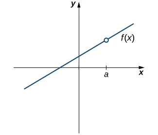
Figure 2.32 — The function \(f(x)\) is not continuous at a* because \(f(a)\) is undefined.*
Condition (i) alone is not enough. In Figure 2.33, \(f(a)\) is defined, but the function still has a gap there because the two-sided limit \(\lim_{x\to a}f(x)\) does not exist. So we add:
$$ \text{ii.}\ \lim_{x\to a}f(x)\ \text{exists.} $$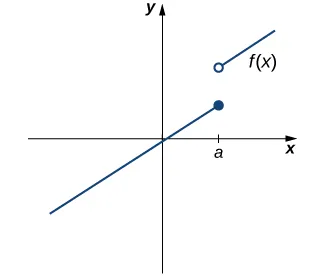
Figure 2.33 — The function \(f(x)\) is not continuous at a* because \(\lim_{x\to a}f(x)\) does not exist.*
Conditions (i) and (ii) together are still not enough. In Figure 2.34 the function value exists, the limit exists — and they disagree. The graph approaches one height but the point sits at another. So we add the final condition:
$$ \text{iii.}\ \lim_{x\to a}f(x)=f(a). $$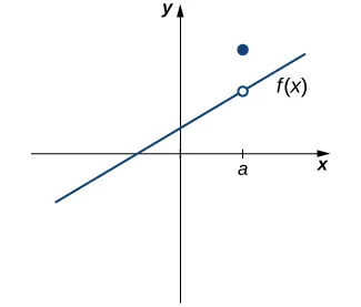
Figure 2.34 — The function \(f(x)\) is not continuous at a* because \(\lim_{x\to a}f(x)\ne f(a).\)*
The next theorem says that for a huge family of familiar functions — polynomials and ratios of polynomials — continuity is automatic everywhere they are defined. We get this for free from the limit laws of the previous section.
Theorem: Continuity of Polynomials and Rational Functions
Polynomials and rational functions are continuous at every point in their domains.
Proof. In the previous section we showed that for any polynomial \(p(x)\), \(\lim_{x\to a}p(x)=p(a)\), and that for a rational function \(\dfrac{p(x)}{q(x)}\) we have \(\lim_{x\to a}\dfrac{p(x)}{q(x)}=\dfrac{p(a)}{q(a)}\) as long as \(q(a)\ne 0\). Both statements say exactly that condition (iii) of Definition 2.1 holds — so each function is continuous everywhere on its domain. \(\square\)
We now apply this theorem to find where a given rational function is continuous.
2.4.2 Types of Discontinuities
If \(f(x)\) is discontinuous at \(a\), then:
- 1. \(f\) has a removable discontinuity at \(a\) if \(\lim_{x\to a}f(x)\) exists. (Here "exists" means \(\lim_{x\to a}f(x)=L\) for some real number \(L\) — not \(\pm\infty\).)
- 2. \(f\) has a jump discontinuity at \(a\) if \(\lim_{x\to a^-}f(x)\) and \(\lim_{x\to a^+}f(x)\) both exist (as real numbers, not \(\pm\infty\)), but \(\lim_{x\to a^-}f(x)\ne\lim_{x\to a^+}f(x)\).
- 3. \(f\) has an infinite discontinuity at \(a\) if \(\lim_{x\to a^-}f(x)=\pm\infty\) and/or \(\lim_{x\to a^+}f(x)=\pm\infty\).
As we have already seen in Examples 2.1 and 2.2, discontinuities don't all look alike. We sort them into three named flavors:
- A removable discontinuity is a hole — the limit exists, but either the function is undefined there or the function value sits at the wrong height.
- A jump discontinuity is a step — the function approaches different heights from the left and the right.
- An infinite discontinuity is a vertical asymptote — the function blows up to \(\pm\infty\) from at least one side.
The classification hinges entirely on what \(\lim_{x\to a}f(x)\) does. If the two-sided limit exists (finite), the break is removable — you could redefine \(f(a)\) to patch it. If the one-sided limits exist but disagree, the break is a jump. If at least one one-sided limit blows up, the break is infinite. Compute the limit first, then read off the label.
Figure 2.37 puts the three pictures side by side. These names cover the cases you'll see most often, but be aware: not every discontinuity fits neatly into one of these three boxes (oscillating breaks, for instance, are their own beast).
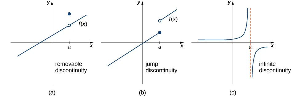
Figure 2.37 — Discontinuities are classified as (a) removable, (b) jump, or (c) infinite.
The formal definition collects the three cases:
2.4.3 Continuity over an Interval
Continuity at a single point is the right opening move. The real-world question, though, is usually "is the function continuous over this whole stretch?" — the kind of statement we need before applying theorems like the Intermediate Value Theorem later in the section. Picture the pencil-trace test again: a function is continuous over an interval if you can drag the pencil from one end to the other without ever lifting it. The complication is what happens at the endpoints of a closed interval, and that's where one-sided continuity comes in.
Continuity from the Right and from the Left
A function \(f(x)\) is continuous from the right at \(a\) if \(\lim_{x\to a^+}f(x)=f(a).\)
A function \(f(x)\) is continuous from the left at \(a\) if \(\lim_{x\to a^-}f(x)=f(a).\)
A function is continuous over an open interval \((a,b)\) if it is continuous at every point in the interval. A function \(f(x)\) is continuous over a closed interval \([a,b]\) if it is continuous at every point in \((a,b)\) and is continuous from the right at \(a\) and is continuous from the left at \(b\). Continuity over a half-open interval like \((a,b]\) is defined analogously: continuous over \((a,b)\) and continuous from the left at \(b\). Other interval shapes work the same way — match the side of the endpoint to the side of the limit.
Why the one-sided requirements at endpoints? Approaching \(a\) from outside the interval doesn't make sense — there's nothing to approach from. The right-hand requirement at \(a\) and the left-hand requirement at \(b\) are exactly what we need so the pencil can start at \(\bigl(a,f(a)\bigr)\) and finish at \(\bigl(b,f(b)\bigr)\) without ever lifting. If, say, \(\lim_{x\to a^+}f(x)\ne f(a)\), the very first stroke would already require a lift.
The next theorem lets us push limits through a continuous outer function. This is the engine we'll use to prove the trig functions are continuous everywhere on their domains.
Theorem: Composite Function Theorem
If \(f(x)\) is continuous at \(L\) and \(\lim_{x\to a}g(x)=L\), then
$$ \lim_{x\to a}f\bigl(g(x)\bigr)=f\!\left(\lim_{x\to a}g(x)\right)=f(L). $$
In words: when the outer function is continuous at the destination, the limit symbol slides inside the outer function. We can compute the inner limit first, then plug it in.
Before we use it, recall from the limit-laws section that \(\lim_{x\to 0}\cos x=1=\cos(0)\), so \(\cos x\) is continuous at \(0\). The next example pairs that fact with the composite function theorem.
The Composite Function Theorem, combined with the continuity of \(\sin x\) and \(\cos x\) at \(0\), unlocks the next theorem — trig functions are continuous everywhere they are defined.
Theorem: Continuity of Trigonometric Functions
Trigonometric functions are continuous over their entire domains.
Proof (cosine case). We show \(\lim_{x\to a}\cos x=\cos a\) for every real \(a\). Use the angle-sum identity \(\cos(u+v)=\cos u\cos v-\sin u\sin v\) with \(u=x-a\) and \(v=a\):
$$ \begin{aligned} \lim_{x\to a}\cos x &=\lim_{x\to a}\cos\bigl((x-a)+a\bigr) \\ &=\lim_{x\to a}\bigl(\cos(x-a)\cos a-\sin(x-a)\sin a\bigr) \\ &=\cos\!\left(\lim_{x\to a}(x-a)\right)\cos a-\sin\!\left(\lim_{x\to a}(x-a)\right)\sin a \\ &=\cos(0)\cos a-\sin(0)\sin a \\ &=1\cdot\cos a-0\cdot\sin a=\cos a. \end{aligned} $$The pivot at step 3 is the Composite Function Theorem applied to \(\sin\) and \(\cos\) at \(0\), where both are continuous. The proof for \(\sin x\) is analogous. The remaining trig functions are quotients of sine and cosine, so their continuity (on their domains) follows from the quotient limit law. \(\square\)
The composite function theorem is one of those small theorems that keeps showing up. We will reach for it again and again as we work with chained-together functions.
2.4.4 The Intermediate Value Theorem
A function that is continuous over a closed interval inherits a whole bundle of useful properties. The first of these — and one of the most useful theorems in single-variable calculus — is the Intermediate Value Theorem. The idea is intuitive: if you trace the graph from \(\bigl(a,f(a)\bigr)\) to \(\bigl(b,f(b)\bigr)\) without lifting your pencil, you must pass through every horizontal level between \(f(a)\) and \(f(b)\) somewhere along the way.
Theorem: The Intermediate Value Theorem (IVT)
Let \(f\) be continuous over a closed, bounded interval \([a,b]\). If \(z\) is any real number between \(f(a)\) and \(f(b)\), then there is a number \(c\) in \([a,b]\) satisfying \(f(c)=z\).
The IVT is an existence theorem — it guarantees a \(c\) exists, but it doesn't tell you which value of \(c\) works, and it doesn't tell you that there's only one. The most common application: pick \(z=0\) and use the IVT to prove an equation has a solution.
Problem Set 2.4
For the following exercises, determine the point(s), if any, at which each function is discontinuous. Classify any discontinuity as jump, removable, infinite, or other.
Problem 30. \(f(x)=\dfrac{1}{\sqrt{x}}\)
Problem 31. \(f(x)=\dfrac{2}{x^2+1}\)
Problem 32. \(f(x)=\dfrac{x}{x^2-x}\)
Problem 33. \(g(t)=t^{-1}+1\)
Problem 34. \(f(x)=\dfrac{5}{e^x-2}\)
Problem 35. \(f(x)=\dfrac{|x-2|}{x-2}\)
Problem 36. \(H(x)=\tan 2x\)
Problem 37. \(f(t)=\dfrac{t+3}{t^2+5t+6}\)
Solutions 1–8
Problem 1
Step 1 — Identify the domain: The expression \(\dfrac{1}{\sqrt{x}}\) requires \(\sqrt{x}\) to be defined and nonzero, so we need \(x>0\). The natural domain is \((0,\infty)\).
Step 2 — Check behavior at boundary points: For \(x<0\), \(f\) is not defined (no real square root). At \(x=0\), \(f\) is undefined and \(\sqrt{x}\to 0^+\), so
$$\lim_{x\to 0^+}\frac{1}{\sqrt{x}}=+\infty.$$Step 3 — Classify: Since one-sided behavior at \(0\) is infinite (and the function is not defined on the left), \(x=0\) is an infinite discontinuity. On \((0,\infty)\), \(f\) is continuous as a composition of continuous functions.
Answer: Infinite discontinuity at \(x=0\); continuous on \((0,\infty)\).
Problem 2
Step 1 — Examine the denominator: \(x^2+1\ge 1>0\) for every real \(x\), so the denominator never vanishes.
Step 2 — Apply continuity of rational functions: \(f(x)=\dfrac{2}{x^2+1}\) is a rational function whose denominator has no real roots, hence \(f\) is continuous on all of \(\mathbb{R}\).
Answer: No discontinuities; \(f\) is continuous on \((-\infty,\infty)\).
Problem 3
Step 1 — Factor the denominator: \(x^2-x=x(x-1)\), so
$$f(x)=\frac{x}{x(x-1)}.$$The denominator is zero at \(x=0\) and \(x=1\); these are the candidate discontinuities.
Step 2 — Simplify and classify \(x=0\): For \(x\ne 0\), \(f(x)=\dfrac{1}{x-1}\). Then
$$\lim_{x\to 0}f(x)=\lim_{x\to 0}\frac{1}{x-1}=-1,$$a finite limit, but \(f(0)\) is undefined. This is a removable discontinuity at \(x=0\).
Step 3 — Classify \(x=1\): Near \(x=1\), \(\dfrac{1}{x-1}\to+\infty\) from the right and \(-\infty\) from the left, so
$$\lim_{x\to 1^+}f(x)=+\infty,\qquad \lim_{x\to 1^-}f(x)=-\infty.$$This is an infinite discontinuity at \(x=1\).
Answer: Removable discontinuity at \(x=0\); infinite discontinuity at \(x=1\).
Problem 4
Step 1 — Rewrite: \(g(t)=t^{-1}+1=\dfrac{1}{t}+1\). The only candidate for discontinuity is \(t=0\), where \(g\) is undefined.
Step 2 — Take one-sided limits at \(t=0\):
$$\lim_{t\to 0^+}\left(\frac{1}{t}+1\right)=+\infty,\qquad \lim_{t\to 0^-}\left(\frac{1}{t}+1\right)=-\infty.$$Step 3 — Classify: Both one-sided limits are infinite, so \(t=0\) is an infinite discontinuity.
Answer: Infinite discontinuity at \(t=0\); continuous on \((-\infty,0)\cup(0,\infty)\).
Problem 5
Step 1 — Locate denominator zeros: Set \(e^x-2=0\), giving \(e^x=2\), so \(x=\ln 2\). Elsewhere \(e^x-2\ne 0\) and the numerator \(5\) is constant.
Step 2 — Analyze one-sided behavior at \(x=\ln 2\): As \(x\to\ln 2^+\), \(e^x>2\), so \(e^x-2\to 0^+\) and \(\dfrac{5}{e^x-2}\to+\infty\). As \(x\to\ln 2^-\), \(e^x<2\), so \(e^x-2\to 0^-\) and \(\dfrac{5}{e^x-2}\to-\infty\).
Step 3 — Classify: Infinite discontinuity at \(x=\ln 2\). Elsewhere, \(f\) is continuous as a quotient of continuous functions with nonzero denominator.
Answer: Infinite discontinuity at \(x=\ln 2\).
Problem 6
Step 1 — Identify the candidate: The denominator \(x-2\) is zero at \(x=2\); the numerator \(|x-2|\) is also zero there, but \(f(2)\) is undefined.
Step 2 — Compute one-sided limits at \(x=2\): For \(x>2\), \(|x-2|=x-2\), so \(f(x)=1\) and \(\lim_{x\to 2^+}f(x)=1\). For \(x<2\), \(|x-2|=-(x-2)\), so \(f(x)=-1\) and \(\lim_{x\to 2^-}f(x)=-1\).
Step 3 — Classify: Both one-sided limits exist as finite numbers but disagree (\(1\ne -1\)). This is a jump discontinuity at \(x=2\).
Answer: Jump discontinuity at \(x=2\).
Problem 7
Step 1 — Rewrite \(\tan 2x\): \(H(x)=\dfrac{\sin 2x}{\cos 2x}\) is undefined where \(\cos 2x=0\), i.e. when \(2x=\dfrac{\pi}{2}+k\pi\) for integer \(k\), giving
$$x=\frac{\pi}{4}+\frac{k\pi}{2},\quad k\in\mathbb{Z}.$$Step 2 — Behavior at each such \(x\): Near these points, \(\cos 2x\to 0\) while \(\sin 2x=\pm 1\ne 0\), so \(H(x)\) blows up to \(\pm\infty\) from either side.
Step 3 — Classify: Each of these points is an infinite discontinuity. Elsewhere \(H\) is continuous as a composition/quotient of continuous functions.
Answer: Infinite discontinuities at \(x=\dfrac{\pi}{4}+\dfrac{k\pi}{2}\) for every integer \(k\).
Problem 8
Step 1 — Factor the denominator: \(t^2+5t+6=(t+2)(t+3)\), so
$$f(t)=\frac{t+3}{(t+2)(t+3)}.$$Candidate discontinuities are \(t=-2\) and \(t=-3\).
Step 2 — Classify \(t=-3\): For \(t\ne -3\), \(f(t)=\dfrac{1}{t+2}\). Then
$$\lim_{t\to -3}f(t)=\frac{1}{-3+2}=-1,$$a finite limit, while \(f(-3)\) is undefined. Removable discontinuity at \(t=-3\).
Step 3 — Classify \(t=-2\): \(\dfrac{1}{t+2}\to+\infty\) as \(t\to -2^+\) and \(\to-\infty\) as \(t\to -2^-\). Infinite discontinuity at \(t=-2\).
Answer: Removable discontinuity at \(t=-3\); infinite discontinuity at \(t=-2\).
For the following exercises, decide if the function is continuous at the given point. If it is discontinuous, what type of discontinuity is it?
Problem 38. \(f(x)=\dfrac{2x^2-5x+3}{x-1}\) at \(x=1\)
Problem 39. \(h(\theta)=\dfrac{\sin\theta-\cos\theta}{\tan\theta}\) at \(\theta=\pi\)
Problem 40. \(g(u)=\begin{cases}\dfrac{6u^2+u-2}{2u-1} & \text{if } u\ne \dfrac{1}{2} \\ \dfrac{7}{2} & \text{if } u=\dfrac{1}{2}\end{cases}\), at \(u=\dfrac{1}{2}\)
Problem 41. \(f(y)=\dfrac{\sin(\pi y)}{\tan(\pi y)}\), at \(y=1\)
Problem 42. \(f(x)=\begin{cases}x^2-e^x & \text{if } x<0 \\ x-1 & \text{if } x\ge 0\end{cases}\), at \(x=0\)
Problem 43. \(f(x)=\begin{cases}x\sin(x) & \text{if } x\le \pi \\ x\tan(x) & \text{if } x>\pi\end{cases}\), at \(x=\pi\)
In the following exercises, find the value(s) of \(k\) that makes each function continuous over the given interval.
Problem 44. \(f(x)=\begin{cases}3x+2, & x
Problem 45. \(f(\theta)=\begin{cases}\sin\theta, & 0\le \theta<\dfrac{\pi}{2} \\ \cos(\theta+k), & \dfrac{\pi}{2}\le \theta\le \pi\end{cases}\)
Problem 46. \(f(x)=\begin{cases}\dfrac{x^2+3x+2}{x+2}, & x\ne -2 \\ k, & x=-2\end{cases}\)
Problem 47. \(f(x)=\begin{cases}e^{kx}, & 0\le x<4 \\ x+3, & 4\le x\le 8\end{cases}\)
Problem 48. \(f(x)=\begin{cases}\sqrt{kx}, & 0\le x\le 3 \\ x+1, & 3 In the following exercises, use the Intermediate Value Theorem (IVT).
Problem 49. Let \(h(x)=\begin{cases}3x^2-4, & x\le 2 \\ 5+4x, & x>2\end{cases}\). Over the interval \([0,4]\), there is no value of \(x\) such that \(h(x)=10\), although \(h(0)<10\) and \(h(4)>10\). Explain why this does not contradict the IVT.
Problem 50. A particle moving along a line has at each time \(t\) a position function \(s(t)\), which is continuous. Assume \(s(2)=5\) and \(s(5)=2\). Another particle moves such that its position is given by \(h(t)=s(t)-t\). Explain why there must be a value \(c\) for \(2
Problem 51. [T] Use the statement "The cosine of \(t\) is equal to \(t\) cubed."
a) Write a mathematical equation of the statement.
b) Prove that the equation in part a. has at least one real solution.
c) Use a calculator to find an interval of length 0.01 that contains a solution.
Problem 52. Apply the IVT to determine whether \(2^x=x^3\) has a solution in one of the intervals \([1.25,1.375]\) or \([1.375,1.5]\). Briefly explain your response for each interval.
Problem 53. Consider the graph of the function \(y=f(x)\) shown in the following graph.
a) Find all values for which the function is discontinuous.
b) For each value in part a., state why the formal definition of continuity does not apply.
c) Classify each discontinuity as either jump, removable, or infinite.
![Exercise figure for 2.4.24 — a continuous curved function over the interval [a,b].](../images/figure_ex_2.4.154.png)
Problem 54. Let \(f(x)=\begin{cases}3x, & x>1 \\ x^3, & x<1\end{cases}\).
a) Sketch the graph of \(f\).
b) Is it possible to find a value \(k\) such that \(f(1)=k\), which makes \(f(x)\) continuous for all real numbers? Briefly explain.
Problem 55. Let \(f(x)=\dfrac{x^4-1}{x^2-1}\) for \(x\ne -1, 1\).
a) Sketch the graph of \(f\).
b) Is it possible to find values \(k_1\) and \(k_2\) such that \(f(-1)=k_1\) and \(f(1)=k_2\), and that makes \(f(x)\) continuous for all real numbers? Briefly explain.
Problem 56. Sketch the graph of a function \(y=f(x)\) with properties i. through vi.
i. The domain of \(f\) is \((-\infty,+\infty)\).
ii. \(f\) has an infinite discontinuity at \(x=-6\).
iii. \(f(-6)=3\).
iv. \(\lim_{x\to -3^-}f(x)=\lim_{x\to -3^+}f(x)=2\).
v. \(f(-3)=3\).
vi. \(f\) is left continuous but not right continuous at \(x=3\).
Problem 57. Sketch the graph of a function \(y=f(x)\) with properties i. through iv.
i. The domain of \(f\) is \([0,5]\).
ii. \(\lim_{x\to 1^+}f(x)\) and \(\lim_{x\to 1^-}f(x)\) exist and are equal.
iii. \(f(x)\) is left continuous but not continuous at \(x=2\), and right continuous but not continuous at \(x=3\).
iv. \(f(x)\) has a removable discontinuity at \(x=1\), a jump discontinuity at \(x=2\), and the following limits hold: \(\lim_{x\to 3^-}f(x)=-\infty\) and \(\lim_{x\to 3^+}f(x)=2\).
In the following exercises, suppose \(y=f(x)\) is defined for all \(x\). For each description, sketch a graph with the indicated property.
Problem 58. Discontinuous at \(x=1\) with \(\lim_{x\to -1}f(x)=-1\) and \(\lim_{x\to 2}f(x)=4\).
Problem 59. Discontinuous at \(x=2\) but continuous elsewhere with \(\lim_{x\to 0}f(x)=\dfrac{1}{2}\).
Determine whether each of the given statements is true. Justify your response with an explanation or counterexample.
Problem 60. \(f(t)=\dfrac{2}{e^t-e^{-t}}\) is continuous everywhere.
Problem 61. If the left- and right-hand limits of \(f(x)\) as \(x\to a\) exist and are equal, then \(f\) cannot be discontinuous at \(x=a\).
Problem 62. If a function is not continuous at a point, then it is not defined at that point.
Problem 63. According to the IVT, \(\cos x-\sin x-x=2\) has a solution over the interval \([-1,1]\).
Problem 64. If \(f(x)\) is continuous such that \(f(a)\) and \(f(b)\) have opposite signs, then \(f(x)=0\) has exactly one solution in \([a,b]\).
Problem 65. The function \(f(x)=\dfrac{x^2-4x+3}{x^2-1}\) is continuous over the interval \([0,3]\).
Problem 66. If \(f(x)\) is continuous everywhere and \(f(a), f(b)>0\), then there is no root of \(f(x)\) in the interval \([a,b]\).
[T] The following problems consider the scalar form of Coulomb's law, which describes the electrostatic force between two point charges, such as electrons. It is given by the equation \(F(r)=k_e\dfrac{|q_1 q_2|}{r^2}\), where \(k_e\) is Coulomb's constant, \(q_i\) are the magnitudes of the charges of the two particles, and \(r\) is the distance between the two particles.
Problem 67. To simplify the calculation of a model with many interacting particles, after some threshold value \(r=R\), we approximate \(F\) as zero.
a) Explain the physical reasoning behind this assumption.
b) What is the force equation?
c) Evaluate the force \(F\) using both Coulomb's law and our approximation, assuming two protons with a charge magnitude of \(1.6022\times 10^{-19}\) coulombs (C), and the Coulomb constant \(k_e=8.988\times 10^9\;\text{N}\cdot\text{m}^2/\text{C}^2\) are 1 m apart. Also, assume \(R<1\) m. How much inaccuracy does our approximation generate? Is our approximation reasonable?
d) Is there any finite value of \(R\) for which this system remains continuous at \(R\)?
Problem 68. Instead of making the force 0 at \(R\), instead we let the force be \(10^{-20}\) for \(r\ge R\). Assume two protons, which have a magnitude of charge \(1.6022\times 10^{-19}\) C, and the Coulomb constant \(k_e=8.988\times 10^9\;\text{N}\cdot\text{m}^2/\text{C}^2\). Is there a value \(R\) that can make this system continuous? If so, find it.
Recall the discussion on spacecraft from the chapter opener. The following problems consider a rocket launch from Earth's surface. The force of gravity on the rocket is given by \(F(d)=-mk/d^2\), where \(m\) is the mass of the rocket, \(d\) is the distance of the rocket from the center of Earth, and \(k\) is a constant.
Problem 69. [T] Determine the value and units of \(k\) given that the mass of the rocket is 3 million kg. (Hint: The distance from the center of Earth to its surface is 6378 km.)
Problem 70. [T] After a certain distance \(D\) has passed, the gravitational effect of Earth becomes quite negligible, so we can approximate the force function by \(F(d)=\begin{cases}-\dfrac{mk}{d^2} & \text{if } d
Problem 71. As the rocket travels away from Earth's surface, there is a distance \(D\) where the rocket sheds some of its mass, since it no longer needs the excess fuel storage. We can write this function as \(F(d)=\begin{cases}-\dfrac{m_1 k}{d^2} & \text{if } d Prove the following functions are continuous everywhere.
Problem 72. \(f(\theta)=\sin\theta\)
Problem 73. \(g(x)=|x|\)
Problem 74. Where is \(f(x)=\begin{cases}0 & \text{if } x \text{ is irrational} \\ 1 & \text{if } x \text{ is rational}\end{cases}\) continuous?
Solutions 9–45
Problem 9
Step 1 — Check the value: \(f(1)\) requires dividing by \(1-1=0\), so \(f(1)\) is undefined and continuity at \(x=1\) fails.
Step 2 — Factor and simplify: \(2x^2-5x+3=(2x-3)(x-1)\), so for \(x\ne 1\)
$$f(x)=\frac{(2x-3)(x-1)}{x-1}=2x-3.$$Therefore \(\lim_{x\to 1}f(x)=2(1)-3=-1\), a finite real number.
Step 3 — Classify: The limit exists but \(f(1)\) is undefined. This is a removable discontinuity.
Answer: Discontinuous at \(x=1\); the discontinuity is removable.
Problem 10
Step 1 — Evaluate the pieces at \(\theta=\pi\): \(\sin\pi=0\), \(\cos\pi=-1\), and \(\tan\pi=\dfrac{\sin\pi}{\cos\pi}=0\). The denominator is \(0\) while the numerator is \(0-(-1)=1\), so \(h(\pi)\) is undefined and \(h\) is discontinuous at \(\theta=\pi\).
Step 2 — Take one-sided limits: Write \(h(\theta)=\dfrac{\sin\theta-\cos\theta}{\sin\theta/\cos\theta}=\dfrac{(\sin\theta-\cos\theta)\cos\theta}{\sin\theta}\). As \(\theta\to\pi\), the numerator \((\sin\theta-\cos\theta)\cos\theta\to (0-(-1))(-1)=-1\), while \(\sin\theta\to 0\) with \(\sin\theta>0\) for \(\theta\to\pi^-\) and \(\sin\theta<0\) for \(\theta\to\pi^+\). Hence
$$\lim_{\theta\to\pi^-}h(\theta)=-\infty,\qquad \lim_{\theta\to\pi^+}h(\theta)=+\infty.$$Step 3 — Classify: One-sided limits are infinite, so this is an infinite discontinuity at \(\theta=\pi\).
Answer: Discontinuous at \(\theta=\pi\); infinite discontinuity.
Problem 11
Step 1 — Compute the limit as \(u\to\tfrac{1}{2}\): Factor the numerator: \(6u^2+u-2=(2u-1)(3u+2)\). Then for \(u\ne\tfrac{1}{2}\),
$$\frac{6u^2+u-2}{2u-1}=\frac{(2u-1)(3u+2)}{2u-1}=3u+2.$$So \(\lim_{u\to 1/2}g(u)=3\cdot\tfrac{1}{2}+2=\tfrac{7}{2}\).
Step 2 — Compare to the defined value: \(g\!\left(\tfrac{1}{2}\right)=\tfrac{7}{2}\), which matches the limit.
Step 3 — Conclude: The limit equals the function value, so \(g\) is continuous at \(u=\tfrac{1}{2}\).
Answer: Continuous at \(u=\dfrac{1}{2}\).
Problem 12
Step 1 — Evaluate at \(y=1\): \(\sin(\pi)=0\) and \(\tan(\pi)=0\), so \(f(1)\) is undefined — \(f\) is discontinuous at \(y=1\).
Step 2 — Simplify and take the limit: For values of \(y\) near \(1\) with \(\sin(\pi y)\ne 0\),
$$f(y)=\frac{\sin(\pi y)}{\tan(\pi y)}=\frac{\sin(\pi y)\cos(\pi y)}{\sin(\pi y)}=\cos(\pi y).$$Hence \(\lim_{y\to 1}f(y)=\cos\pi=-1\), a finite real number.
Step 3 — Classify: Limit exists but \(f(1)\) is undefined — removable discontinuity.
Answer: Discontinuous at \(y=1\); the discontinuity is removable.
Problem 13
Step 1 — Compute \(f(0)\): Since \(0\ge 0\), use the second piece: \(f(0)=0-1=-1\).
Step 2 — Take one-sided limits at \(x=0\):
$$\lim_{x\to 0^-}f(x)=\lim_{x\to 0^-}(x^2-e^x)=0-1=-1,$$ $$\lim_{x\to 0^+}f(x)=\lim_{x\to 0^+}(x-1)=-1.$$Step 3 — Conclude: Both one-sided limits equal \(-1=f(0)\), so \(\lim_{x\to 0}f(x)=f(0)\) and \(f\) is continuous at \(x=0\).
Answer: Continuous at \(x=0\).
Problem 14
Step 1 — Compute \(f(\pi)\): Since \(\pi\le\pi\), use the first piece: \(f(\pi)=\pi\sin\pi=\pi\cdot 0=0\).
Step 2 — Left-hand limit:
$$\lim_{x\to\pi^-}f(x)=\lim_{x\to\pi^-}x\sin x=\pi\sin\pi=0.$$Step 3 — Right-hand limit:
$$\lim_{x\to\pi^+}f(x)=\lim_{x\to\pi^+}x\tan x=\pi\tan\pi=\pi\cdot 0=0.$$Step 4 — Compare: Both one-sided limits equal \(0=f(\pi)\), so \(\lim_{x\to\pi}f(x)=f(\pi)\) and \(f\) is continuous at \(x=\pi\).
Answer: Continuous at \(x=\pi\).
Problem 15
Step 1 — Identify where continuity could fail: Each branch is a polynomial, hence continuous on its domain. The only candidate for discontinuity is the boundary \(x=k\), where the rule switches from \(3x+2\) to \(2x-3\).
Step 2 — Force the one-sided limits to agree: At \(x=k\) the left limit is \(\lim_{x\to k^-}(3x+2)=3k+2\), and the function value (also the right limit) is \(2k-3\). Continuity at \(k\) requires
$$3k+2=2k-3.$$Step 3 — Solve for \(k\): Subtract \(2k\) from both sides: \(k+2=-3\), so \(k=-5\).
Answer: \(k=-5\).
Problem 16
Step 1 — Locate the seam: Both \(\sin\theta\) and \(\cos(\theta+k)\) are continuous everywhere; we only need to match values at \(\theta=\pi/2\).
Step 2 — Match the two branches: The left-hand limit is \(\sin(\pi/2)=1\). The right-hand value is \(\cos(\pi/2+k)=-\sin k\). Continuity requires
$$-\sin k = 1, \quad \text{i.e.,} \quad \sin k = -1.$$Step 3 — Solve for \(k\): The general solution is \(k=-\dfrac{\pi}{2}+2\pi n\) for any integer \(n\). The simplest choice is \(k=-\dfrac{\pi}{2}\).
Answer: \(k=-\dfrac{\pi}{2}+2\pi n\) for integer \(n\); typically \(k=-\dfrac{\pi}{2}\).
Problem 17
Step 1 — Simplify the rational expression: Factor the numerator:
$$\frac{x^2+3x+2}{x+2}=\frac{(x+1)(x+2)}{x+2}=x+1 \quad (x\ne -2).$$Step 2 — Compute the limit at the trouble point: \(\lim_{x\to -2}(x+1)=-1\).
Step 3 — Match \(f(-2)\) to the limit: Continuity at \(-2\) requires \(f(-2)=k=-1\).
Answer: \(k=-1\).
Problem 18
Step 1 — Identify the seam: Both branches are continuous on their pieces. Match values at \(x=4\).
Step 2 — Set up the matching equation: The left limit is \(\lim_{x\to 4^-}e^{kx}=e^{4k}\); the right value is \(4+3=7\). Continuity requires
$$e^{4k}=7.$$Step 3 — Solve for \(k\): Take the natural log of both sides:
$$4k=\ln 7 \quad\Longrightarrow\quad k=\frac{\ln 7}{4}.$$Answer: \(k=\dfrac{\ln 7}{4}\).
Problem 19
Step 1 — Identify the seam: Both pieces are continuous on their respective intervals (assuming \(kx\ge 0\) on \([0,3]\)). Match values at \(x=3\).
Step 2 — Set up the matching equation: The left value is \(\sqrt{3k}\); the right limit is \(3+1=4\). Continuity requires
$$\sqrt{3k}=4.$$Step 3 — Solve for \(k\): Square both sides: \(3k=16\), so \(k=\dfrac{16}{3}\). Check: \(k>0\) keeps the radicand non-negative on \([0,3]\).
Answer: \(k=\dfrac{16}{3}\).
Problem 20
Step 1 — Check continuity of \(h\) on \([0,4]\): At the seam \(x=2\), the left value is \(h(2)=3(4)-4=8\); the right limit is \(\lim_{x\to 2^+}(5+4x)=13\). These disagree, so \(h\) has a jump discontinuity at \(x=2\).
Step 2 — State the IVT hypothesis: The IVT requires the function to be continuous on the closed interval. Here \(h\) is not continuous on \([0,4]\) because of the jump at \(x=2\).
Step 3 — Reconcile: Although \(h(0)=-4<10\) and \(h(4)=21>10\), the values between \(8\) and \(13\) (in particular \(10\)) are skipped over by the jump and are never attained. The IVT's conclusion is not contradicted because its hypothesis (continuity on the closed interval) fails.
Answer: The IVT requires continuity on the entire closed interval, and \(h\) is discontinuous at \(x=2\). With the hypothesis broken, the IVT makes no prediction, so there is no contradiction.
Problem 21
Step 1 — Establish continuity of \(h\): Since \(s(t)\) is continuous and \(t\) is continuous, the difference \(h(t)=s(t)-t\) is continuous on \([2,5]\).
Step 2 — Evaluate at the endpoints:
$$h(2)=s(2)-2=5-2=3>0,$$ $$h(5)=s(5)-5=2-5=-3<0.$$Step 3 — Apply the IVT: Because \(h\) is continuous on \([2,5]\) and \(h(2)>0>h(5)\), the value \(0\) lies between \(h(2)\) and \(h(5)\). The IVT guarantees a \(c\in(2,5)\) with \(h(c)=0\) (equivalently, \(s(c)=c\)).
Answer: By the IVT applied to the continuous function \(h\) on \([2,5]\), some \(c\in(2,5)\) satisfies \(h(c)=0\).
Problem 22
Step 1 — (a) Write the equation: "Cosine of \(t\) equals \(t\) cubed" gives
$$\cos t = t^3.$$Step 2 — (b) Build an auxiliary continuous function: Let \(g(t)=\cos t - t^3\). Then \(g\) is continuous on \(\mathbb{R}\) (cosine and polynomials are continuous). Evaluate at convenient endpoints:
$$g(0)=\cos 0 - 0 = 1>0,$$ $$g(1)=\cos 1 - 1 \approx 0.5403-1 = -0.4597<0.$$Since \(g\) is continuous on \([0,1]\) and changes sign, the IVT guarantees a \(c\in(0,1)\) with \(g(c)=0\), i.e., \(\cos c = c^3\).
Step 3 — (c) Narrow to an interval of length 0.01: Bisect repeatedly. Using a calculator,
- \(g(0.86)=\cos(0.86)-0.86^3\approx 0.6518-0.6361\approx 0.0157>0\), - \(g(0.87)=\cos(0.87)-0.87^3\approx 0.6442-0.6585\approx -0.0143<0\).
The sign change places a root in \([0.86,0.87]\), an interval of length \(0.01\).
Answer: (a) \(\cos t=t^3\); (b) by the IVT on \(g(t)=\cos t-t^3\) over \([0,1]\), a solution exists; (c) a solution lies in \([0.86, 0.87]\).
Problem 23
Step 1 — Set up the test function: Let \(g(x)=2^x-x^3\). Both \(2^x\) and \(x^3\) are continuous, so \(g\) is continuous everywhere. A root of \(g\) corresponds to a solution of \(2^x=x^3\).
Step 2 — Test \([1.25, 1.375]\):
- \(g(1.25)=2^{1.25}-1.25^3 \approx 2.3784-1.9531\approx 0.4253>0\), - \(g(1.375)=2^{1.375}-1.375^3 \approx 2.5937-2.5996\approx -0.0059<0\).
Sign change present, so by IVT there is a solution in \([1.25,1.375]\).
Step 3 — Test \([1.375, 1.5]\):
- \(g(1.375)\approx -0.0059<0\), - \(g(1.5)=2^{1.5}-1.5^{3}\approx 2.8284-3.3750\approx -0.5466<0\).
No sign change, so the IVT yields no conclusion here (a root may or may not exist, but this test does not detect one).
Answer: A solution exists in \([1.25, 1.375]\) by the IVT (sign change). The IVT does not guarantee a solution in \([1.375, 1.5]\) since \(g\) has the same sign at both endpoints.
Problem 24
Step 1 — Inspect the provided figure: The figure accompanying this section illustrates the IVT: a single continuous curve drawn over an interval \([a,b]\) with no breaks, holes, jumps, or vertical asymptotes shown. Every point on the curve is a single well-defined value of \(f\).
Step 2 — (a) List discontinuities: Based strictly on what is depicted, there are no points of discontinuity to report — the function shown is continuous on its visible domain \([a,b]\).
Step 3 — (b) Why the formal definition does not flag any point: At every \(x\) shown, the limit exists and equals \(f(x)\); all three conditions of the formal definition (\(f(x)\) defined, \(\lim_{t\to x}f(t)\) exists, and the two are equal) hold throughout, so none of them can be used to identify a discontinuity.
Step 4 — (c) Classification: With no discontinuities present, there is nothing to classify. (For reference: had the graph shown an open/filled-point pair at a single \(x\), that would be removable; a vertical gap between two pieces would be jump; a vertical asymptote would be infinite.)
Answer: The figure shows a continuous curve, so (a) there are no discontinuities, (b) the definition is satisfied everywhere visible, and (c) there is nothing to classify.
Problem 25
Step 1 — (a) Describe the graph: For \(x<1\), draw the cubic \(y=x^3\); it passes through \((-1,-1)\) and approaches the point \((1,1)\) as \(x\to 1^-\) (open circle at \((1,1)\)). For \(x>1\), draw the line \(y=3x\); as \(x\to 1^+\), \(y\to 3\) (open circle at \((1,3)\)). At \(x=1\) the function is currently undefined.
Step 2 — Examine the one-sided limits at \(x=1\):
$$\lim_{x\to 1^-}f(x)=\lim_{x\to 1^-}x^3=1, \qquad \lim_{x\to 1^+}f(x)=\lim_{x\to 1^+}3x=3.$$These are not equal, so \(\lim_{x\to 1}f(x)\) does not exist.
Step 3 — (b) Decide whether one \(k\) can repair continuity: Continuity at \(x=1\) requires \(\lim_{x\to 1}f(x)\) to exist and equal \(f(1)=k\). Since the two one-sided limits disagree (a jump), no single value of \(k\) can make \(f\) continuous at \(x=1\).
Answer: (a) Cubic on the left, line \(y=3x\) on the right, with a jump at \(x=1\) (open circles at \((1,1)\) and \((1,3)\)). (b) No such \(k\) exists; the one-sided limits at \(1\) differ.
Problem 26
Step 1 — Simplify the formula: Factor the numerator as a difference of squares:
$$\frac{x^4-1}{x^2-1}=\frac{(x^2-1)(x^2+1)}{x^2-1}=x^2+1\quad (x\ne \pm 1).$$Step 2 — (a) Describe the graph: The graph is the upward parabola \(y=x^2+1\) (vertex at \((0,1)\)), but with open circles at \((-1,2)\) and \((1,2)\) since \(f\) is undefined there.
Step 3 — Compute the limits at the holes:
$$\lim_{x\to -1}(x^2+1)=2,\qquad \lim_{x\to 1}(x^2+1)=2.$$Step 4 — (b) Choose \(k_1\) and \(k_2\): Both discontinuities are removable. Setting \(f(-1)=k_1=2\) and \(f(1)=k_2=2\) fills in the holes so that \(f(x)=x^2+1\) on all of \(\mathbb{R}\), which is continuous everywhere.
Answer: (a) The parabola \(y=x^2+1\) with open holes at \((-1,2)\) and \((1,2)\). (b) Yes: \(k_1=k_2=2\) removes both discontinuities.
Problem 27
Step 1 — Inventory the requirements: domain \((-\infty,\infty)\); infinite discontinuity at \(x=-6\) with \(f(-6)=3\); a removable-style scenario at \(x=-3\) where the two-sided limit equals \(2\) but \(f(-3)=3\); at \(x=3\) the function is left-continuous but not right-continuous.
Step 2 — Build a verbal sketch: To the left of \(x=-6\), draw a curve plunging down (or shooting up) to a vertical asymptote at \(x=-6\); to the right of \(x=-6\), another branch coming back from the opposite infinity. Mark the single point \((-6, 3)\) as a filled dot floating off the curve (the function is defined there even though the limit blows up). Continue smoothly toward \(x=-3\): the curve approaches the point \((-3, 2)\) from both sides (open circle at \((-3,2)\)) while a filled dot sits at \((-3,3)\) above it — a removable discontinuity with \(f(-3)\) reassigned. Continue smoothly to \(x=3\). At \(x=3\), the left branch arrives at a filled dot at \((3, y_0)\) for some chosen \(y_0\); the right branch starts at an open circle at \((3, y_1)\) with \(y_1\ne y_0\) and proceeds rightward. Because the filled value equals the left limit, \(f\) is left-continuous at 3 but not right-continuous.
Step 3 — Verify each property in turn: 1. Domain \((-\infty,\infty)\): every \(x\) has a function value (the asymptote at \(x=-6\) is "filled" by the dot at height 3). 2. Infinite discontinuity at \(x=-6\): vertical asymptote present. 3. \(f(-6)=3\): the floating dot. 4. \(\lim_{x\to -3}f(x)=2\) from both sides: the curve closes on \((-3,2)\). 5. \(f(-3)=3\): the dot above the hole. 6. At \(x=3\): left limit equals \(f(3)\) (left-continuous), right limit differs (jump on the right).
Answer: A sketch with a vertical asymptote at \(x=-6\) (with an isolated dot at \((-6,3)\)), a removable-style hole at \(x=-3\) where the curve approaches \(y=2\) but \(f(-3)=3\), and a jump at \(x=3\) where the left piece closes onto \(f(3)\) (filled) and the right piece starts at a different height (open).
Problem 28
Step 1 — Inventory the requirements: domain \([0,5]\); a removable discontinuity at \(x=1\) (two-sided limit exists and matches itself, but \(f(1)\) sits elsewhere); a jump at \(x=2\) where \(f\) is left-continuous; at \(x=3\), \(f\) is right-continuous, the left-hand limit is \(-\infty\), and the right-hand limit is \(2\).
Step 2 — Build a verbal sketch: Start at \(x=0\) with any value, say \((0,1)\). Draw any continuous curve from \(x=0\) to \(x=1\), arriving at an open circle at \((1, L)\) for some value \(L\). Place a separate filled dot at \((1, L')\) with \(L'\ne L\): the limit exists (= \(L\)), but \(f(1)=L'\), giving a removable discontinuity. Continue from the open circle smoothly to \(x=2\), closing onto a filled dot at \((2, M)\) (left-continuous). To the right of \(x=2\), restart at an open circle at \((2, M')\) with \(M'\ne M\) and draw a curve heading toward \(x=3\), descending to \(-\infty\) (vertical asymptote at \(x=3\) on the left). For \(x>3\), the curve starts at a filled dot at \((3, 2)\) (right-continuous, matches the right limit) and continues to \(x=5\).
Step 3 — Verify each property: 1. Domain \([0,5]\): values exist on the whole interval (including filled dots at \(1\), \(2\), and \(3\)). 2. \(\lim_{x\to 1^\pm}f(x)=L\): both one-sided limits land at the open circle at height \(L\). 3. At \(x=2\): left limit \(=M=f(2)\) (left-continuous), right limit \(=M'\ne M\) (not right-continuous), so jump. 4. At \(x=3\): left limit \(=-\infty\); \(f(3)=2\) matches the right limit \(2\) (right-continuous, not left-continuous). 5. Removable at \(1\), jump at \(2\), \(-\infty\) versus \(2\) at \(3\): all accounted for.
Answer: A sketch on \([0,5]\) with a hole-and-dot pair at \(x=1\) (removable), a left-closed/right-open jump at \(x=2\), and a leftward vertical asymptote (down to \(-\infty\)) at \(x=3\) paired with a filled dot at \((3,2)\) starting the right branch.
Problem 29
Step 1 — Read off the requirements: \(f\) must be discontinuous at \(x=1\), and have specified two-sided limits \(\lim_{x\to -1}f(x)=-1\) and \(\lim_{x\to 2}f(x)=4\) (the function is otherwise continuous at \(-1\) and \(2\)).
Step 2 — Describe a sketch that satisfies all three: Draw any continuous curve that passes through \((-1,-1)\) and \((2,4)\) (for example, a smooth curve sloping upward from lower left through \((-1,-1)\), continuing up through \((2,4)\)). At \(x=1\), break the curve: leave an open circle on the curve at \((1, y_L)\) where the curve "wanted" to go, and place a filled dot at \((1, y_D)\) with \(y_D\ne y_L\) (for example, the curve passes through height 2 at \(x=1\) but you set \(f(1)=5\)). This produces a removable-style discontinuity at \(x=1\) while leaving the limits at \(-1\) and \(2\) untouched.
Step 3 — Verify the conditions: 1. \(\lim_{x\to -1}f(x)=-1\): the curve passes continuously through \((-1,-1)\). 2. \(\lim_{x\to 2}f(x)=4\): the curve passes continuously through \((2,4)\). 3. Discontinuous at \(x=1\): the open circle / filled dot mismatch breaks continuity there.
Answer: Any continuous curve through \((-1,-1)\) and \((2,4)\) with a hole-and-dot mismatch (removable discontinuity) at \(x=1\) — for example, the curve heading through \((1,2)\) but with \(f(1)=5\) marked as a filled dot above the open circle.
Problem 30
Step 1 — Read off the requirements: \(f\) is continuous everywhere except at \(x=2\), and \(\lim_{x\to 0}f(x)=\dfrac{1}{2}\).
Step 2 — Describe a sketch: Draw a smooth curve that passes continuously through \(\left(0,\tfrac{1}{2}\right)\) — for example, a gently rising curve through that point. Extend it smoothly in both directions, keeping it continuous everywhere. At \(x=2\), introduce a single discontinuity: the simplest is a jump (close the left piece with a filled dot at \((2, a)\), restart the right piece with an open circle at \((2, b)\) where \(b\ne a\)). Alternatively, a removable hole or a vertical asymptote at \(x=2\) is acceptable. Outside \(x=2\), the curve has no other breaks.
Step 3 — Verify the conditions: 1. Continuous everywhere except \(x=2\): the only break is the constructed one at \(x=2\). 2. \(\lim_{x\to 0}f(x)=\tfrac{1}{2}\): the smooth curve passes through \(\left(0,\tfrac{1}{2}\right)\), so the limit equals the value.
Answer: A smooth continuous curve passing through \(\left(0,\tfrac{1}{2}\right)\) with exactly one discontinuity at \(x=2\) — for instance, a jump where the left piece closes at \((2,1)\) (filled) and the right piece restarts at \((2,3)\) (open).
Problem 31
Step 1 — Locate the trouble spot: The function \(f(t)=\dfrac{2}{e^{t}-e^{-t}}\) is built from continuous pieces, so it is continuous wherever the denominator is nonzero.
Step 2 — Test the denominator: Set \(e^{t}-e^{-t}=0\). This gives \(e^{t}=e^{-t}\), so \(e^{2t}=1\), hence \(t=0\). At \(t=0\) the function is undefined, so \(f\) is discontinuous there.
Answer: FALSE. \(f\) is undefined (and hence discontinuous) at \(t=0\).
Problem 32
Step 1 — Recall the full definition of continuity at \(x=a\): \(f\) is continuous at \(a\) iff (i) \(f(a)\) is defined, (ii) \(\lim_{x\to a}f(x)\) exists, and (iii) \(\lim_{x\to a}f(x)=f(a)\).
Step 2 — Spot the missing condition: Equal one-sided limits give only (ii). Either \(f(a)\) may be undefined, or it may equal a different value from the limit (a removable discontinuity).
Step 3 — Counterexample: Let \(f(x)=\dfrac{x^{2}-1}{x-1}\). The two-sided limit at \(x=1\) is \(2\), but \(f(1)\) is undefined, so \(f\) is discontinuous at \(1\).
Answer: FALSE.
Problem 33
Step 1 — Possible failure modes: Continuity can fail because \(f(a)\) is undefined, the limit fails to exist, or the limit exists but disagrees with \(f(a)\). Only the first failure mode requires \(f\) to be undefined.
Step 2 — Counterexample: Define
$$f(x)=\begin{cases}1 & x\ne 0\\ 0 & x=0\end{cases}$$Here \(f(0)=0\) is defined, yet \(\lim_{x\to 0}f(x)=1\ne f(0)\), so \(f\) is discontinuous at \(0\).
Answer: FALSE.
Problem 34
Step 1 — Set up an IVT-friendly function: Let \(g(x)=\cos x-\sin x-x-2\). We want a root of \(g\) on \([-1,1]\).
Step 2 — Continuity: \(g\) is a sum of continuous functions, hence continuous on \([-1,1]\).
Step 3 — Endpoint values:
\(g(-1)=\cos(-1)-\sin(-1)-(-1)-2=\cos 1+\sin 1-1\approx 0.5403+0.8415-1\approx 0.382>0\).
\(g(1)=\cos 1-\sin 1-1-2\approx 0.5403-0.8415-3\approx -3.301<0\).
Step 4 — Apply IVT: \(g\) changes sign on \([-1,1]\), so by the Intermediate Value Theorem there exists \(c\in(-1,1)\) with \(g(c)=0\), i.e. \(\cos c-\sin c-c=2\).
Answer: TRUE.
Problem 35
Step 1 — What IVT actually guarantees: Opposite signs at the endpoints of a continuous function guarantee at least one root, not exactly one.
Step 2 — Counterexample: Take \(f(x)=\sin x\) on \([-\,\pi/2,\,3\pi/2]\). Then \(f(-\pi/2)=-1<0\) and \(f(3\pi/2)=-1<0\)… (need opposite signs). Use instead \(f(x)=\sin x\) on \([-\,\pi/2,\,5\pi/2]\): \(f(-\pi/2)=-1\), \(f(5\pi/2)=1\) — opposite signs, but \(\sin x=0\) has roots at \(0,\pi,2\pi\) inside the interval, i.e. three solutions.
Answer: FALSE — there is at least one solution, but possibly more.
Problem 36
Step 1 — Identify discontinuities: \(f(x)=\dfrac{x^{2}-4x+3}{x^{2}-1}\) is a rational function, continuous except where the denominator is zero, i.e. \(x=\pm 1\).
Step 2 — Check the interval: \(x=1\) lies in \([0,3]\), and \(f(1)\) is undefined there.
Answer: FALSE. \(f\) is discontinuous at \(x=1\in[0,3]\).
Problem 37
Step 1 — Sign alone doesn't preclude roots: Same-sign endpoints don't prevent the function from dipping (or rising) through zero between them.
Step 2 — Counterexample: Let \(f(x)=x^{2}-1\) on \([-2,2]\). Then \(f(-2)=3>0\) and \(f(2)=3>0\), yet \(f\) has roots at \(x=\pm 1\) inside \([-2,2]\).
Answer: FALSE.
Problem 38
Part (a) — Physical reasoning: Coulomb force falls off as \(1/r^{2}\), so beyond a chosen cutoff \(R\) the force on any one particle from a distant particle is negligibly small. In a many-particle simulation, ignoring contributions past \(R\) saves an enormous amount of computation while changing each pairwise force by an amount swamped by other modeling errors.
Part (b) — Piecewise force equation:
$$F(r)=\begin{cases}\,k_{e}\dfrac{|q_{1}q_{2}|}{r^{2}} & 0Compute \((1.6022\times 10^{-19})^{2}\approx 2.567\times 10^{-38}\), so
$$F\approx (8.988\times 10^{9})(2.567\times 10^{-38})\approx 2.307\times 10^{-28}\;\text{N}.$$Under the approximation, \(F=0\). The absolute inaccuracy is about \(2.3\times 10^{-28}\) N — utterly negligible compared with any macroscopically meaningful force. The approximation is reasonable.
Part (d) — Continuity at \(R\): For the piecewise \(F\) to be continuous at \(R\) we would need
$$\lim_{r\to R^{-}}k_{e}\dfrac{|q_{1}q_{2}|}{r^{2}}=k_{e}\dfrac{|q_{1}q_{2}|}{R^{2}}=0.$$But \(k_{e}|q_{1}q_{2}|/R^{2}\) is strictly positive for any finite \(R\) (with nonzero charges), so equality with 0 is impossible.
Answer: No finite \(R\) makes the truncated-at-zero model continuous.
Problem 39
Step 1 — Continuity condition at \(r=R\): With
$$F(r)=\begin{cases}k_{e}\dfrac{|q_{1}q_{2}|}{r^{2}} & rStep 2 — Plug in proton charges: \(|q_{1}q_{2}|=(1.6022\times 10^{-19})^{2}\approx 2.567\times 10^{-38}\) C\(^{2}\). Then
$$k_{e}|q_{1}q_{2}|=(8.988\times 10^{9})(2.567\times 10^{-38})\approx 2.307\times 10^{-28}\;\text{N}\cdot\text{m}^{2}.$$Step 3 — Solve for \(R\):
$$R^{2}=\dfrac{k_{e}|q_{1}q_{2}|}{10^{-20}}=\dfrac{2.307\times 10^{-28}}{10^{-20}}=2.307\times 10^{-8}\;\text{m}^{2},$$ $$R=\sqrt{2.307\times 10^{-8}}\approx 1.519\times 10^{-4}\;\text{m}.$$Answer: Yes — choose \(R\approx 1.52\times 10^{-4}\) m \((\approx 0.152\) mm\()\).
Problem 40
Step 1 — Set up the equation: At Earth's surface (\(d=R_{\oplus}=6378\) km \(=6.378\times 10^{6}\) m), the gravitational force on the rocket equals its weight: \(-mk/R_{\oplus}^{2}=-mg\).
Step 2 — Solve for \(k\): The masses cancel:
$$k=g\,R_{\oplus}^{2}=(9.8)(6.378\times 10^{6})^{2}.$$Compute \((6.378\times 10^{6})^{2}\approx 4.068\times 10^{13}\). Then
$$k\approx (9.8)(4.068\times 10^{13})\approx 3.986\times 10^{14}\;\text{m}^{3}/\text{s}^{2}.$$Step 3 — Units check: \([g][R^{2}]=(\text{m}/\text{s}^{2})(\text{m}^{2})=\text{m}^{3}/\text{s}^{2}\). Consistent with the standard gravitational parameter \(GM_{\oplus}\).
Note on the graphing calculator: Entering \(9.8\times (6378000)^{2}\) on a TI-style calculator returns approximately \(3.986\times 10^{14}\), which a graph of \(k=g\,R^{2}\) at \(R=6378\) km would also show as a horizontal value of the same magnitude.
Answer: \(k\approx 3.986\times 10^{14}\;\text{m}^{3}/\text{s}^{2}\).
Problem 41
Step 1 — Continuity condition at \(d=D\): With \(m=3\times 10^{6}\) kg and \(k\approx 3.986\times 10^{14}\) m\(^{3}\)/s\(^{2}\), continuity requires
$$-\dfrac{mk}{D^{2}}=10{,}000.$$Step 2 — Solve for \(D\): Take absolute values (the left side is negative, but matching magnitudes in the limit setup; setting the algebraic equality gives the same \(D\) up to sign of the constant — proceed with magnitudes):
$$D^{2}=\dfrac{mk}{10{,}000}=\dfrac{(3\times 10^{6})(3.986\times 10^{14})}{10^{4}}.$$Numerator: \((3\times 10^{6})(3.986\times 10^{14})\approx 1.196\times 10^{21}\). Divide by \(10^{4}\):
$$D^{2}\approx 1.196\times 10^{17}\;\text{m}^{2},\qquad D\approx 3.458\times 10^{8}\;\text{m}.$$Step 3 — Sanity check: \(3.458\times 10^{8}\) m is roughly the Earth–Moon distance scale (\(\sim 3.84\times 10^{8}\) m), which is physically plausible for "gravity becomes negligible at the \(10^{4}\) N level for a 3-million-kg rocket."
Note on the graphing calculator: Plotting \(y=-mk/d^{2}\) and \(y=10{,}000\) on the same axes and intersecting (or using the solver on \(mk/d^{2}=10{,}000\)) returns \(D\approx 3.46\times 10^{8}\) m.
Answer: \(D\approx 3.46\times 10^{8}\) m.
Problem 42
Step 1 — Continuity condition at \(D\): Equality of one-sided limits requires
$$-\dfrac{m_{1}k}{D^{2}}=-\dfrac{m_{2}k}{D^{2}}.$$Step 2 — Simplify: Cancel \(-k/D^{2}\) (nonzero for any finite \(D>0\)). The equation reduces to \(m_{1}=m_{2}\).
Step 3 — Contradict the hypothesis: We are told \(m_{1}\ne m_{2}\), so the equality cannot hold for any finite \(D\).
Answer: No — for \(m_{1}\ne m_{2}\), the piecewise \(F\) has a jump at every finite \(D\) and so cannot be made continuous.
Problem 43
Step 1 — Goal: Show \(\lim_{x\to a}\sin x=\sin a\) for every real \(a\).
Step 2 — Substitute \(x=a+h\): As \(x\to a\), \(h=x-a\to 0\). The composition \(h(x)=x-a\) is continuous, and the limit becomes \(\lim_{h\to 0}\sin(a+h)\).
Step 3 — Angle-sum identity:
$$\sin(a+h)=\sin a\cos h+\cos a\sin h.$$Step 4 — Use continuity of \(\sin\) and \(\cos\) at \(0\): From the section, \(\lim_{h\to 0}\cos h=1\) and \(\lim_{h\to 0}\sin h=0\). By the sum and product laws for limits,
$$\lim_{h\to 0}\sin(a+h)=\sin a\cdot 1+\cos a\cdot 0=\sin a.$$Step 5 — Apply the Composite Function Theorem: Since \(h(x)=x-a\) is continuous at \(a\) with \(h(a)=0\), and \(\sin\) is continuous at \(0\) (the chain through which we evaluated), the composition gives \(\lim_{x\to a}\sin x=\sin a\).
Answer: \(\sin\theta\) is continuous at every real \(a\), hence continuous everywhere.
Problem 44
Step 1 — Case \(a>0\): For \(x\) near \(a\), \(x>0\) and so \(|x|=x\). Then \(\lim_{x\to a}|x|=\lim_{x\to a}x=a=|a|\).
Step 2 — Case \(a<0\): For \(x\) near \(a\), \(x<0\) and so \(|x|=-x\). Then \(\lim_{x\to a}|x|=\lim_{x\to a}(-x)=-a=|a|\).
Step 3 — Case \(a=0\): Use one-sided limits.
Right-hand: for \(x>0\), \(|x|=x\), so \(\lim_{x\to 0^{+}}|x|=\lim_{x\to 0^{+}}x=0\).
Left-hand: for \(x<0\), \(|x|=-x\), so \(\lim_{x\to 0^{-}}|x|=\lim_{x\to 0^{-}}(-x)=0\).
Both one-sided limits equal \(0=|0|\), so \(\lim_{x\to 0}|x|=0=|0|\).
Step 4 — Conclude: In every case, \(\lim_{x\to a}|x|=|a|\), so \(g(x)=|x|\) is continuous at every real \(a\).
Answer: \(g(x)=|x|\) is continuous on \((-\infty,\infty)\).
Problem 45
Step 1 — Density facts: Every nonempty open interval contains both rational and irrational numbers (the rationals and irrationals are each dense in \(\mathbb{R}\)).
Step 2 — Test continuity at an arbitrary \(a\): Fix any real \(a\). In every deleted neighborhood of \(a\) we can pick a sequence of rationals \(x_{n}\to a\), giving \(f(x_{n})=1\to 1\), and a sequence of irrationals \(y_{n}\to a\), giving \(f(y_{n})=0\to 0\).
Step 3 — Limit cannot exist: Two sequences approaching \(a\) produce different limits (\(1\) and \(0\)), so \(\lim_{x\to a}f(x)\) does not exist. Hence \(f\) is discontinuous at \(a\).
Step 4 — \(a\) was arbitrary: The argument did not depend on whether \(a\) was rational or irrational.
Answer: \(f\) is discontinuous at every real number — i.e. \(f\) is continuous nowhere.
Key Terms
continuous at a point — \(f(a)\) is defined, \(\lim_{x\to a}f(x)\) exists, and the two are equal.
discontinuous at a point — \(f\) fails at least one of the three conditions for continuity at \(a\).
removable discontinuity — a discontinuity at \(a\) where \(\lim_{x\to a}f(x)\) exists as a real number; can be repaired by redefining \(f(a)\).
jump discontinuity — a discontinuity where the one-sided limits both exist (as real numbers) but disagree.
infinite discontinuity — a discontinuity where at least one one-sided limit is \(\pm\infty\); corresponds to a vertical asymptote.
continuous from the right at \(a\) — \(\lim_{x\to a^+}f(x)=f(a)\).
continuous from the left at \(a\) — \(\lim_{x\to a^-}f(x)=f(a)\).
continuity over an interval — continuous at every interior point and (for closed/half-closed intervals) one-sided continuous at each included endpoint.
Composite Function Theorem — if \(f\) is continuous at \(L\) and \(\lim_{x\to a}g(x)=L\), then \(\lim_{x\to a}f(g(x))=f(L)\).
Intermediate Value Theorem (IVT) — if \(f\) is continuous on \([a,b]\) and \(z\) lies between \(f(a)\) and \(f(b)\), there exists \(c\in[a,b]\) with \(f(c)=z\).