Chapter 3
3.1 Defining the Derivative
Learning Objectives
- Recognize the meaning of the tangent to a curve at a point.
- Calculate the slope of a tangent line.
- Identify the derivative as the limit of a difference quotient.
- Calculate the derivative of a given function at a point.
- Describe the velocity as a rate of change.
- Explain the difference between average velocity and instantaneous velocity.
- Estimate the derivative from a table of values.
Now that we have both a conceptual understanding of limits and the practical ability to compute them, we have the foundation to study calculus — the branch of mathematics built on derivatives and integrals. Most mathematicians and historians agree that calculus was developed independently by the Englishman Isaac Newton (1643–1727) and the German Gottfried Leibniz (1646–1716), whose images appear in Figure 3.2.
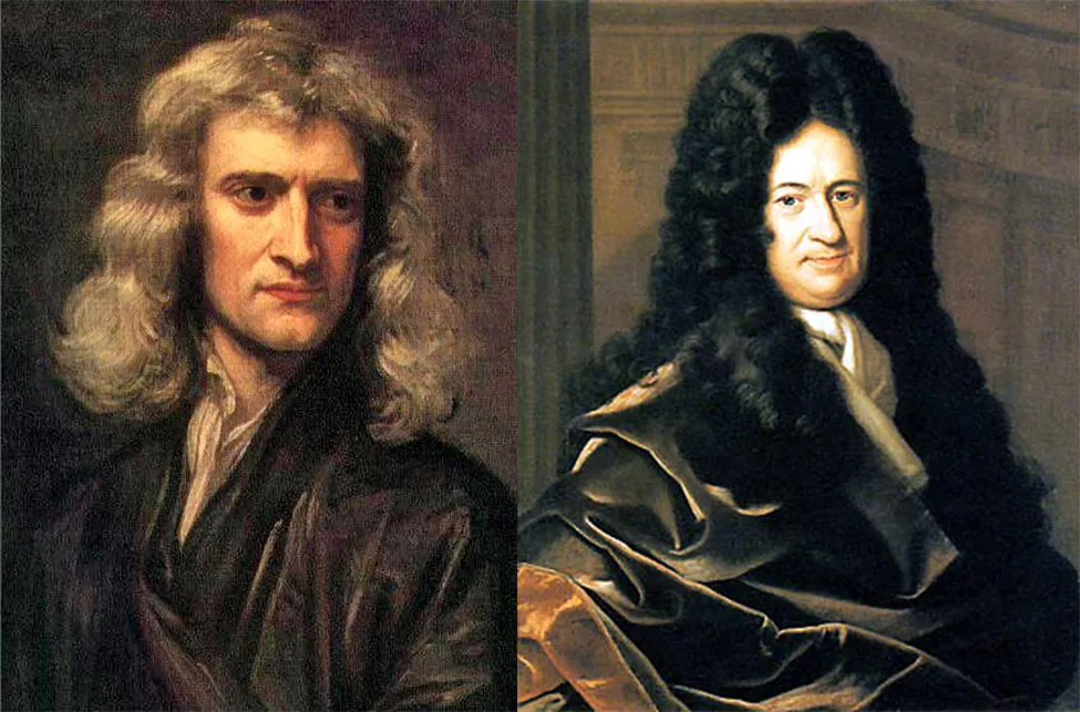
Figure 3.2 — Newton and Leibniz are credited with developing calculus independently.
When we credit Newton and Leibniz with developing calculus, we mean they were the first to understand the deep relationship between the derivative and the integral. Both built on the work of predecessors such as Barrow, Fermat, and Cavalieri. The initial relationship between the two mathematicians was amicable; in later years a bitter priority dispute erupted. It seems likely Newton arrived at the core ideas first, but we owe Leibniz the notation we use today.
3.1.1 Tangent Lines
Let \(f\) be a function defined on an interval \(I\) containing \(a.\) If \(x \ne a\) is in \(I,\) then
$$Q = \frac{f(x) - f(a)}{x - a}$$is a difference quotient.
Also, if \(h \ne 0\) is chosen so that \(a + h\) is in \(I,\) then
$$Q = \frac{f(a+h) - f(a)}{h}$$is a difference quotient with increment \(h.\)
Media
These two expressions for the secant slope are illustrated in Figure 3.3. Both are useful; the choice usually comes down to whichever makes the algebra easier.
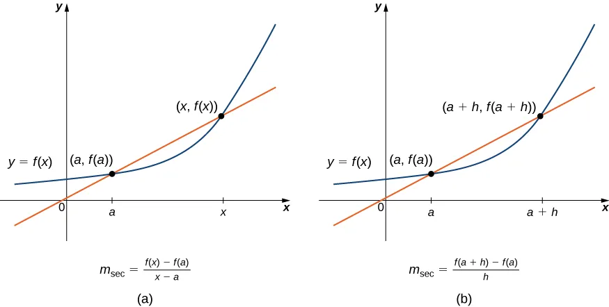
Figure 3.3 — We can calculate the slope of a secant line in either of two ways.
In Figure 3.4(a) we see that as the values of \(x\) approach \(a,\) the secant lines approach the tangent line to \(f\) at \(a.\) In Figure 3.4(b) the same convergence appears as \(h \to 0.\) The slope of the tangent line at \(a\) is the instantaneous rate of change of \(f\) at \(a,\) shown in Figure 3.4(c).
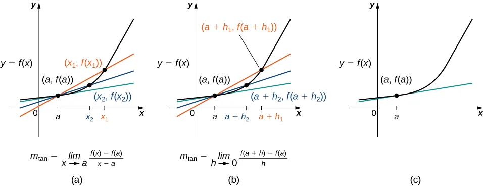
Figure 3.4 — The secant lines approach the tangent line (shown in green) as the second point approaches the first.
Media
Why do we care about the tangent line? Because it gives us the "true" local slope — the instantaneous slope of a curve at one precise point. A secant line is an average: it uses two points. As the second point gets closer and closer to the first, the secant slope closes in on the tangent slope. This limiting process — taking a secant slope to its limit — is the geometric heart of differentiation.
In Figure 3.5 we show the graph of \(f(x) = \sqrt{x}\) and its tangent line at \((1, 1)\) in increasingly tight windows about \(x = 1.\) As the windows narrow, the curve and its tangent line appear to coincide — the function looks locally linear near \(x = 1.\)
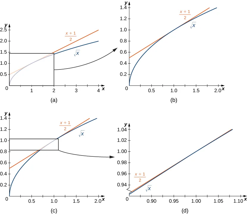
Figure 3.5 — For values of \(x\) close to \(1,\) the graph of \(f(x) = \sqrt{x}\) and its tangent line appear to coincide.
Formally, the tangent line is defined as a limit:
Let \(f(x)\) be a function defined in an open interval containing \(a.\) The tangent line to \(f(x)\) at \(a\) is the line passing through \((a, f(a))\) with slope
$$m_{\tan} = \lim_{x \to a} \frac{f(x) - f(a)}{x - a}$$provided this limit exists.
Equivalently, the tangent line has slope
$$m_{\tan} = \lim_{h \to 0} \frac{f(a+h) - f(a)}{h}$$provided this limit exists.
Just as we have two difference-quotient forms for the secant slope, we use both forms for the tangent slope. Either may be used; the choice depends on ease of calculation. Now let's use this definition to find tangent line equations.
We begin by revisiting secant lines and tangent lines. Recall that the slope of a secant line to a function \(f\) at a point \((a, f(a))\) estimates the rate of change. We pick a second value of \(x\) near \(a\) and draw the line through \((a, f(a))\) and \((x, f(x)),\) as shown in Figure 3.3. That slope is the difference quotient:
$$m_{\sec} = \frac{f(x) - f(a)}{x - a}.$$We can also write the secant slope using an increment \(h\) (where \(h\) is close to 0), setting the second point at \((a+h,\, f(a+h)):\)
$$m_{\sec} = \frac{f(a+h) - f(a)}{h}.$$Find the slope of the line tangent to the graph of \(f(x) = \sqrt{x}\) at \(x = 4.\)
Solution
Step 1 — Set up the limit using Equation 3.3:
$$m_{\tan} = \lim_{x \to 4} \frac{\sqrt{x} - 2}{x - 4}$$This is a \(\tfrac{0}{0}\) indeterminate form. Multiply by the conjugate of the numerator.
Step 2 — Multiply numerator and denominator by \((\sqrt{x} + 2):\)
$$m_{\tan} = \lim_{x \to 4} \frac{(\sqrt{x} - 2)(\sqrt{x} + 2)}{(x - 4)(\sqrt{x} + 2)} = \lim_{x \to 4} \frac{x - 4}{(x - 4)(\sqrt{x} + 2)}$$Step 3 — Cancel and evaluate:
$$= \lim_{x \to 4} \frac{1}{\sqrt{x} + 2} = \frac{1}{\sqrt{4} + 2} = \frac{1}{4}$$Answer: The slope of the tangent line at \(x = 4\) is \(\dfrac{1}{4}.\)
Find an equation of the line tangent to the graph of \(f(x) = x^2\) at \(x = 3.\)
Solution
Step 1 — Find the slope using Equation 3.3:
$$\begin{array}{rcll} m_{\tan} & = & \displaystyle\lim_{x \to 3} \frac{f(x) - f(3)}{x - 3} & \text{Apply the definition.} \\[10pt] & = & \displaystyle\lim_{x \to 3} \frac{x^2 - 9}{x - 3} & \text{Substitute } f(x) = x^2 \text{ and } f(3) = 9. \\[10pt] & = & \displaystyle\lim_{x \to 3} \frac{(x-3)(x+3)}{x-3} & \text{Factor the numerator.} \\[10pt] & = & \displaystyle\lim_{x \to 3} (x + 3) = 6 & \text{Cancel and evaluate.} \end{array}$$Step 2 — Identify a point on the tangent line:
The tangent touches the curve at \(x = 3,\) so we use the point \((3,\, f(3)) = (3, 9).\)
Step 3 — Write the equation using point-slope form:
$$y - 9 = 6(x - 3) \implies y = 6x - 9$$The graph of \(f(x) = x^2\) and its tangent line are shown in Figure 3.6.
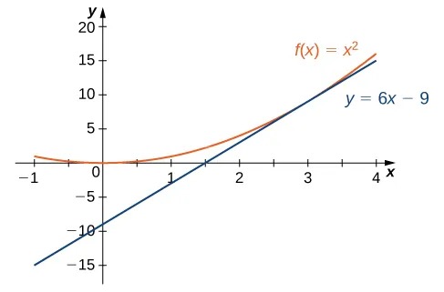
Figure 3.6 — The tangent line to \(f(x)\) at \(x = 3.\)
Answer: \(y = 6x - 9\)
Use Equation 3.4 to find the slope of the line tangent to the graph of \(f(x) = x^2\) at \(x = 3.\)
Solution
The steps closely parallel Example 3.1.1, but now we use the \(h\)-increment form.
$$\begin{array}{rcll} m_{\tan} & = & \displaystyle\lim_{h \to 0} \frac{f(3+h) - f(3)}{h} & \text{Apply the definition.} \\[10pt] & = & \displaystyle\lim_{h \to 0} \frac{(3+h)^2 - 9}{h} & \text{Substitute } f(3+h) = (3+h)^2 \text{ and } f(3) = 9. \\[10pt] & = & \displaystyle\lim_{h \to 0} \frac{9 + 6h + h^2 - 9}{h} & \text{Expand } (3+h)^2. \\[10pt] & = & \displaystyle\lim_{h \to 0} \frac{h(6 + h)}{h} & \text{Factor out } h. \\[10pt] & = & \displaystyle\lim_{h \to 0} (6 + h) = 6 & \text{Cancel and evaluate.} \end{array}$$Answer: \(m_{\tan} = 6,\) confirming Example 3.1.1. The two forms of the definition always produce the same answer — choose whichever is more convenient.
Find an equation of the line tangent to the graph of \(f(x) = \dfrac{1}{x}\) at \(x = 2.\)
Solution
Step 1 — Find the slope using Equation 3.3:
$$\begin{array}{rcll} m_{\tan} & = & \displaystyle\lim_{x \to 2} \frac{f(x) - f(2)}{x - 2} & \text{Apply the definition.} \\[10pt] & = & \displaystyle\lim_{x \to 2} \frac{\dfrac{1}{x} - \dfrac{1}{2}}{x - 2} & \text{Substitute } f(x) = \dfrac{1}{x} \text{ and } f(2) = \dfrac{1}{2}. \\[10pt] & = & \displaystyle\lim_{x \to 2} \frac{\dfrac{1}{x} - \dfrac{1}{2}}{x - 2} \cdot \frac{2x}{2x} & \text{Multiply by } \dfrac{2x}{2x} \text{ to clear fractions.} \\[10pt] & = & \displaystyle\lim_{x \to 2} \frac{2 - x}{(x-2)(2x)} & \text{Simplify the numerator.} \\[10pt] & = & \displaystyle\lim_{x \to 2} \frac{-1}{2x} & \text{Use } \dfrac{2-x}{x-2} = -1 \text{ for } x \neq 2. \\[10pt] & = & -\dfrac{1}{4} & \text{Evaluate the limit.} \end{array}$$Step 2 — Find a point on the tangent line:
$$f(2) = \frac{1}{2}, \quad \text{so the tangent passes through } \left(2,\, \tfrac{1}{2}\right).$$Step 3 — Write the equation:
$$y - \frac{1}{2} = -\frac{1}{4}(x - 2) \implies y = -\frac{1}{4}x + 1$$The graphs of \(f(x) = \dfrac{1}{x}\) and \(y = -\dfrac{1}{4}x + 1\) are shown in Figure 3.7.
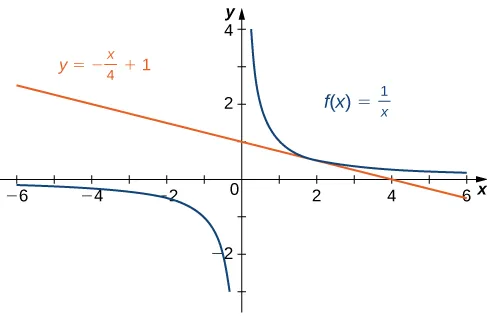
Figure 3.7 — The line is tangent to \(f(x)\) at \(x = 2.\)
Answer: \(y = -\dfrac{1}{4}x + 1\)
3.1.2 The Derivative of a Function at a Point
Let \(f(x)\) be a function defined in an open interval containing \(a.\) The derivative of the function \(f(x)\) at \(a,\) denoted by \(f'(a),\) is defined by
$$f'(a) = \lim_{x \to a} \frac{f(x) - f(a)}{x - a} \qquad \text{(Equation 3.5)}$$provided this limit exists.
Alternatively, we may define the derivative of \(f(x)\) at \(a\) as
$$f'(a) = \lim_{h \to 0} \frac{f(a+h) - f(a)}{h} \qquad \text{(Equation 3.6)}$$provided this limit exists.
Think of the derivative as a speedometer reading. The odometer on your car records total distance traveled — that's the position function. The speedometer shows how fast distance is changing right now — that's the derivative. Average speed over a road trip is like the secant line slope (total change divided by total time); the speedometer reading at any instant is like the tangent line slope, which is the derivative. Every smooth function has a "speedometer reading" at each point, and that reading is exactly \(f'(a).\)
The notation \(f'(a)\) is read "f prime of a." It is a single number — the instantaneous rate of change of \(f\) at the input value \(a.\) Notice that \(f'(a)\) and \(m_{\tan}\) from Definition 3.2 are the same object: the derivative at \(a\) equals the slope of the tangent line at \(a.\)
The slope of a tangent line — the limit we computed in the previous section — appears so often across physics, engineering, economics, and biology that we give it a special name: the derivative. The process of finding a derivative is called differentiation.
For \(f(x) = x^2,\) use a table to estimate \(f'(3)\) using Equation 3.6 (the \(h\)-increment form). Do you get the same estimate as Example 3.1.4?
Solution
We build a table of values of \(\dfrac{f(3+h) - f(3)}{h} = \dfrac{(3+h)^2 - 9}{h}\) for small values of \(h\) approaching \(0.\)
| \(h\) | \(\dfrac{(3+h)^2 - 9}{h}\) |
|---|---|
| \(-0.1\) | 5.9 |
| \(-0.01\) | 5.99 |
| \(-0.001\) | 5.999 |
| \(0.001\) | 6.001 |
| \(0.01\) | 6.01 |
| \(0.1\) | 6.1 |
As \(h \to 0,\) the values again close in on \(6.\)
Answer: \(f'(3) \approx 6,\) confirming Example 3.1.4. The two forms of the definition always agree.
For \(f(x) = x^2,\) use a table to estimate \(f'(3)\) using Equation 3.5.
Solution
We build a table of values of \(\dfrac{f(x) - f(3)}{x - 3} = \dfrac{x^2 - 9}{x - 3}\) for values of \(x\) approaching \(3\) from both sides.
| \(x\) | \(\dfrac{x^2 - 9}{x - 3}\) |
|---|---|
| 2.9 | 5.9 |
| 2.99 | 5.99 |
| 2.999 | 5.999 |
| 3.001 | 6.001 |
| 3.01 | 6.01 |
| 3.1 | 6.1 |
As \(x\) approaches \(3\) from either side, the difference quotient closes in on \(6.\)
Answer: \(f'(3) \approx 6.\) We confirm this exactly in Example 3.1.5.
For \(f(x) = x^2 + 3x + 2,\) find \(f'(1).\)
Solution
Step 1 — Compute \(f(1)\):
$$f(1) = 1 + 3 + 2 = 6$$Step 2 — Apply Equation 3.5:
$$f'(1) = \lim_{x \to 1} \frac{(x^2 + 3x + 2) - 6}{x - 1} = \lim_{x \to 1} \frac{x^2 + 3x - 4}{x - 1}$$Step 3 — Factor and cancel:
$$= \lim_{x \to 1} \frac{(x - 1)(x + 4)}{x - 1} = \lim_{x \to 1} (x + 4) = 5$$Answer: \(f'(1) = 5\)
For \(f(x) = 3x^2 - 4x + 1,\) find \(f'(2)\) by using Equation 3.5.
Solution
First compute \(f(2) = 3(4) - 4(2) + 1 = 12 - 8 + 1 = 5.\)
$$\begin{array}{rcll} f'(2) & = & \displaystyle\lim_{x \to 2} \frac{f(x) - f(2)}{x - 2} & \text{Apply the definition.} \\[10pt] & = & \displaystyle\lim_{x \to 2} \frac{(3x^2 - 4x + 1) - 5}{x - 2} & \text{Substitute } f(x) \text{ and } f(2) = 5. \\[10pt] & = & \displaystyle\lim_{x \to 2} \frac{(x-2)(3x+2)}{x-2} & \text{Factor the numerator.} \\[10pt] & = & \displaystyle\lim_{x \to 2} (3x + 2) & \text{Cancel the common factor.} \\[10pt] & = & 8 & \text{Evaluate the limit.} \end{array}$$Answer: \(f'(2) = 8\)
For \(f(x) = 3x^2 - 4x + 1,\) find \(f'(2)\) by using Equation 3.6.
Solution
We use the \(h\)-form to independently confirm Example 3.1.5.
$$\begin{array}{rcll} f'(2) & = & \displaystyle\lim_{h \to 0} \frac{f(2+h) - f(2)}{h} & \text{Apply the definition.} \\[10pt] & = & \displaystyle\lim_{h \to 0} \frac{\bigl[3(2+h)^2 - 4(2+h) + 1\bigr] - 5}{h} & \text{Substitute and expand.} \\[10pt] & = & \displaystyle\lim_{h \to 0} \frac{3h^2 + 8h}{h} & \text{Simplify; constants cancel.} \\[10pt] & = & \displaystyle\lim_{h \to 0} \frac{h(3h + 8)}{h} & \text{Factor out } h. \\[10pt] & = & \displaystyle\lim_{h \to 0} (3h + 8) = 8 & \text{Cancel and evaluate.} \end{array}$$Answer: \(f'(2) = 8,\) matching Example 3.1.5. The results are the same whether we use Equation 3.5 or Equation 3.6.
3.1.3 Velocities and Rates of Change
The instantaneous rate of change of a function \(f(x)\) at a value \(a\) is its derivative \(f'(a).\)
Now that we can evaluate a derivative, we can apply it to velocity problems. Recall that if \(s(t)\) is the position of an object moving along a coordinate axis, the average velocity over a time interval \([a, t]\) (for \(t > a\)) is
$$v_{\text{ave}} = \frac{s(t) - s(a)}{t - a}.$$As the values of \(t\) approach \(a,\) the average velocities approach the instantaneous velocity at \(a,\) denoted \(v(a)\):
$$v(a) = s'(a) = \lim_{t \to a} \frac{s(t) - s(a)}{t - a}. \qquad \text{(Equation 3.7)}$$In Figure 3.8, the slope of the secant line (green) is the average velocity over \([a, t],\) and the slope of the tangent line (red) is the instantaneous velocity at \(t = a.\)
![Figure 3.8 — The slope of the secant line is the average velocity over the interval \([a,t].\) The slope of the tangent line is the instantaneous velocity.](../images/figure_3.8.png)
Figure 3.8 — The slope of the secant line is the average velocity over the interval \([a,t].\) The slope of the tangent line is the instantaneous velocity.
We can use Equation 3.5 to calculate instantaneous velocity exactly, or we can estimate it from a table of average velocities and then confirm with Equation 3.7.
One of the most tangible applications of the derivative is velocity — measuring how fast an object's position changes at an exact instant.
Here is the unifying picture: slope = rate of change. For a position-vs-time graph, the slope of the secant line between two times is average velocity. The slope of the tangent line at one time is instantaneous velocity. For any function whatsoever, the derivative at a point is the instantaneous rate of change — it doesn't matter whether the function describes distance, temperature, profit, or population. Same formula, same idea, endless applications.
A rock is dropped from a height of \(64\) feet. Its height above ground \(t\) seconds later is given by \(s(t) = -16t^2 + 64\) for \(0 \leq t \leq 2.\) Find the instantaneous velocity \(1\) second after it is dropped using Equation 3.5.
Solution
Step 1 — Compute \(s(1)\):
$$s(1) = -16(1)^2 + 64 = 48 \text{ feet}$$Step 2 — Apply Equation 3.5:
$$v(1) = s'(1) = \lim_{x \to 1} \frac{s(x) - s(1)}{x - 1} = \lim_{x \to 1} \frac{(-16x^2 + 64) - 48}{x - 1} = \lim_{x \to 1} \frac{-16x^2 + 16}{x - 1}$$Step 3 — Factor and cancel:
$$= \lim_{x \to 1} \frac{-16(x^2 - 1)}{x - 1} = \lim_{x \to 1} \frac{-16(x-1)(x+1)}{x-1} = \lim_{x \to 1} -16(x+1) = -32$$Answer: The instantaneous velocity at \(t = 1\) second is \(-32\) ft/s. The negative sign confirms the rock is moving downward.
As we have seen throughout this section, the slope of a tangent line and instantaneous velocity are the same concept viewed in different settings. Each is computed by taking a derivative, and each measures the instantaneous rate of change of a function at a point.
A lead weight on a spring is oscillating up and down. Its position at time \(t\) with respect to a fixed horizontal line is given by \(s(t) = \sin t\) (Figure 3.9). Use a table of values to estimate \(v(0).\) Check the estimate by using Equation 3.5.
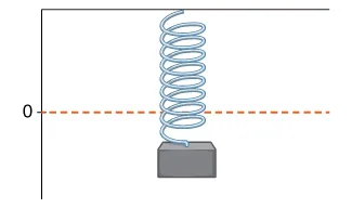
Figure 3.9 — A lead weight suspended from a spring in vertical oscillatory motion.
Solution
Step 1 — Build Table 3.1.1 of average velocities near \(t = 0:\)
We compute \(\dfrac{\sin t - \sin 0}{t - 0} = \dfrac{\sin t}{t}\) for values of \(t\) approaching \(0.\)
| \(t\) | \(\dfrac{\sin t}{t}\) |
|---|---|
| \(-0.1\) | 0.998334166 |
| \(-0.01\) | 0.9999833333 |
| \(-0.001\) | 0.9999998333 |
| \(0.001\) | 0.9999998333 |
| \(0.01\) | 0.9999833333 |
| \(0.1\) | 0.998334166 |
The values approach \(1\) from both sides, so our table estimate is \(v(0) \approx 1.\)
Step 2 — Confirm with Equation 3.5:
$$v(0) = s'(0) = \lim_{t \to 0} \frac{\sin t - \sin 0}{t - 0} = \lim_{t \to 0} \frac{\sin t}{t} = 1$$Answer: \(v(0) = 1\) unit per second.
A coffee shop determines that the daily profit on scones (in dollars) when charging \(s\) dollars per scone is \(P(s) = -20s^2 + 150s - 10.\) The coffee shop currently charges \(\$3.25\) per scone.
a) Find \(P'(3.25),\) the rate of change of profit at this price.
b) Should the coffee shop consider raising or lowering its prices?
Solution
Step 1 — Use Equation 3.6 (the \(h\)-form):
Expand \(P(3.25 + h):\) $$P(3.25 + h) = -20(3.25 + h)^2 + 150(3.25 + h) - 10$$ $$= -20(10.5625 + 6.5h + h^2) + 487.5 + 150h - 10$$ $$= -211.25 - 130h - 20h^2 + 487.5 + 150h - 10 = 266.25 + 20h - 20h^2$$
Since \(P(3.25) = 266.25:\) $$P(3.25 + h) - P(3.25) = h(20 - 20h)$$
$$P'(3.25) = \lim_{h \to 0} \frac{h(20 - 20h)}{h} = \lim_{h \to 0}(20 - 20h) = 20$$Answer:
a) \(P'(3.25) = 20\) dollars of profit per dollar increase in scone price.
b) Since \(P'(3.25) = 20 > 0,\) the coffee shop should raise its prices — at \(\$3.25,\) each small price increase brings in more profit.
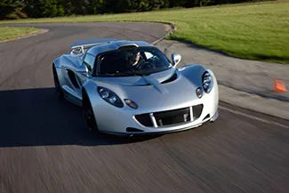
Figure 3.10 — (credit: modification of work by Codex41, Flickr)
Reaching a top speed of \(270.49\) mph, the Hennessey Venom GT is one of the fastest cars in the world. In tests it went from 0 to 60 mph in \(3.05\) seconds, from 0 to 100 mph in \(5.88\) seconds, from 0 to 200 mph in \(14.51\) seconds, and from 0 to 229.9 mph in \(19.96\) seconds. Use this data to draw a conclusion about the rate of change of velocity (that is, its acceleration) as the car approaches \(229.9\) mph. Does the rate at which the car accelerates appear to be increasing, decreasing, or constant?
Solution
Step 1 — Convert speeds to ft/s and organize as Table 3.1.2:
Using \(1 \text{ mph} \approx 1.46\overline{6}\) ft/s:
| \(t\) (sec) | \(v(t)\) (mph) | \(v(t)\) (ft/s) |
|---|---|---|
| 0 | 0 | 0 |
| 3.05 | 60 | 88 |
| 5.88 | 100 | \(\approx 146.67\) |
| 14.51 | 200 | \(\approx 293.33\) |
| 19.96 | 229.9 | \(\approx 337.19\) |
Step 2 — Compute average acceleration on intervals \([t,\, 19.96]\) as Table 3.1.3:
Average acceleration \(= \dfrac{v(19.96) - v(t)}{19.96 - t} = \dfrac{337.19 - v(t)}{19.96 - t}\)
| \(t\) | \(v(t)\) (ft/s) | Avg. acceleration (ft/s²) |
|---|---|---|
| 0 | 0 | \(337.19/19.96 \approx 16.89\) |
| 3.05 | 88 | \(249.19/16.91 \approx 14.74\) |
| 5.88 | 146.67 | \(190.52/14.08 \approx 13.53\) |
| 14.51 | 293.33 | \(43.86/5.45 \approx 8.05\) |
Step 3 — Interpret:
As \(t\) approaches \(19.96\) seconds (when \(v \approx 229.9\) mph), the average acceleration values fall from roughly \(16.89\) to \(8.05\) ft/s².
Answer: The rate at which the car is accelerating is decreasing as its velocity approaches \(229.9\) mph \((\approx 337.19\) ft/s).
A homeowner sets the thermostat so that the temperature in the house begins to drop from \(70°\text{F}\) at 9 p.m., reaches a low of \(60°\) during the night, and rises back to \(70°\) by 7 a.m. Suppose the temperature is given by \(T(t) = 0.4t^2 - 4t + 70\) for \(0 \leq t \leq 10,\) where \(t\) is hours past 9 p.m. Find the instantaneous rate of change of temperature at midnight.
Solution
Midnight is \(3\) hours past 9 p.m., so we want \(T'(3).\)
Step 1 — Compute \(T(3)\):
$$T(3) = 0.4(9) - 4(3) + 70 = 3.6 - 12 + 70 = 61.6°\text{F}$$Step 2 — Apply Equation 3.5:
$$\begin{array}{rcll} T'(3) & = & \displaystyle\lim_{t \to 3} \frac{T(t) - T(3)}{t - 3} & \text{Apply the definition.} \\[10pt] & = & \displaystyle\lim_{t \to 3} \frac{(0.4t^2 - 4t + 70) - 61.6}{t - 3} & \text{Substitute } T(t) \text{ and } T(3) = 61.6. \\[10pt] & = & \displaystyle\lim_{t \to 3} \frac{0.4t^2 - 4t + 8.4}{t - 3} & \text{Simplify.} \\[10pt] & = & \displaystyle\lim_{t \to 3} \frac{0.4(t - 3)(t - 7)}{t - 3} & \text{Factor the numerator.} \\[10pt] & = & \displaystyle\lim_{t \to 3} 0.4(t - 7) & \text{Cancel.} \\[10pt] & = & 0.4(3 - 7) = -1.6 & \text{Evaluate.} \end{array}$$Answer: The instantaneous rate of change of temperature at midnight is \(-1.6°\text{F}\) per hour. The negative sign tells us the temperature is dropping at that moment.
A toy company can sell \(x\) electronic gaming systems at a price of \(p = -0.01x + 400\) dollars per gaming system. The cost of manufacturing \(x\) systems is given by \(C(x) = 100x + 10,000\) dollars. Find the rate of change of profit when \(10,000\) games are produced. Should the toy company increase or decrease production?
Solution
Step 1 — Build the revenue and profit functions:
Revenue is price times quantity: $$R(x) = x \cdot p = x(-0.01x + 400) = -0.01x^2 + 400x$$
Profit is revenue minus cost: $$P(x) = R(x) - C(x) = -0.01x^2 + 400x - 100x - 10,000 = -0.01x^2 + 300x - 10,000$$
Step 2 — Apply Equation 3.5:
$$\begin{array}{rcl} P'(10000) & = & \displaystyle\lim_{x \to 10000} \frac{P(x) - P(10000)}{x - 10000} \\[10pt] & = & \displaystyle\lim_{x \to 10000} \frac{-0.01x^2 + 300x - 10,000 - 1,990,000}{x - 10000} \\[10pt] & = & \displaystyle\lim_{x \to 10000} \frac{-0.01x^2 + 300x - 2,000,000}{x - 10000} \\[10pt] & = & \displaystyle\lim_{x \to 10000} \frac{-0.01(x - 10000)(x - 20000)}{x - 10000} \\[10pt] & = & \displaystyle\lim_{x \to 10000} -0.01(x - 20000) \\[10pt] & = & -0.01(10000 - 20000) = 100 \end{array}$$Step 3 — Interpret:
Since \(P'(10,000) = 100 > 0,\) profit is increasing as production increases at the \(10,000\)-unit level.
Answer: The rate of change of profit is \(\$100\) per system. Since this is positive, the company should increase production.
Problem Set 3.1
Find the derivative of \(f(x) = x^2.\)
Solution
Step 1 — Substitute into Equation 3.7:
$$f'(x) = \lim_{h \to 0} \frac{(x+h)^2 - x^2}{h}$$Step 2 — Expand and simplify:
$$\begin{array}{rcll} & & \displaystyle\lim_{h \to 0} \frac{x^2 + 2xh + h^2 - x^2}{h} & \text{Expand } (x+h)^2. \\[10pt] & = & \displaystyle\lim_{h \to 0} \frac{2xh + h^2}{h} & \text{Cancel } x^2 \text{ terms.} \\[10pt] & = & \displaystyle\lim_{h \to 0} \frac{h(2x + h)}{h} = \lim_{h \to 0}(2x + h) = 2x & \text{Factor and evaluate.} \end{array}$$Answer: \(f'(x) = 2x.\)
Find the derivative of \(f(x) = \sqrt{x}.\)
Solution
Step 1 — Substitute into Equation 3.7:
$$f'(x) = \lim_{h \to 0} \frac{\sqrt{x+h} - \sqrt{x}}{h}$$The numerator is a \(\sqrt{\cdot} - \sqrt{\cdot}\) difference, so the limit is the \(\tfrac{0}{0}\) indeterminate form. The standard trick is to multiply by the conjugate.
Step 2 — Multiply by the conjugate:
$$f'(x) = \lim_{h \to 0} \frac{\sqrt{x+h} - \sqrt{x}}{h} \cdot \frac{\sqrt{x+h} + \sqrt{x}}{\sqrt{x+h} + \sqrt{x}}$$The numerator collapses to a difference of squares: \((\sqrt{x+h})^2 - (\sqrt{x})^2 = (x+h) - x = h.\)
Step 3 — Simplify and cancel the \(h:\)
$$\begin{array}{rcll} f'(x) & = & \displaystyle\lim_{h \to 0} \frac{h}{h(\sqrt{x+h} + \sqrt{x})} & \text{Simplify the numerator.} \\[10pt] & = & \displaystyle\lim_{h \to 0} \frac{1}{\sqrt{x+h} + \sqrt{x}} & \text{Cancel the common factor of } h. \\[10pt] & = & \displaystyle\frac{1}{\sqrt{x} + \sqrt{x}} = \frac{1}{2\sqrt{x}} & \text{Evaluate the limit.} \end{array}$$Answer: \(f'(x) = \dfrac{1}{2\sqrt{x}}.\) Notice the derivative is defined for \(x > 0\) and blows up as \(x \to 0^+\) — the original \(\sqrt{x}\) has a vertical tangent there, so the slope is not finite at \(0.\)
Find the derivative of the function \(f(x) = x^2 - 2x.\)
Solution
No conjugates needed this time — just expand and collect.
Step 1 — Substitute into Equation 3.7:
$$f'(x) = \lim_{h \to 0} \frac{\bigl((x+h)^2 - 2(x+h)\bigr) - (x^2 - 2x)}{h}$$Step 2 — Expand the numerator:
$$\begin{array}{rcll} & & \displaystyle\lim_{h \to 0} \frac{x^2 + 2xh + h^2 - 2x - 2h - x^2 + 2x}{h} & \text{Expand } (x+h)^2 - 2(x+h). \\[10pt] & = & \displaystyle\lim_{h \to 0} \frac{2xh + h^2 - 2h}{h} & \text{Combine like terms.} \\[10pt] & = & \displaystyle\lim_{h \to 0} \frac{h(2x + h - 2)}{h} & \text{Factor out } h. \\[10pt] & = & \displaystyle\lim_{h \to 0} (2x + h - 2) = 2x - 2 & \text{Cancel and evaluate.} \end{array}$$Answer: \(f'(x) = 2x - 2.\) Note that the derivative is itself a polynomial — and it is defined for every real number. Later we'll see this is true of every polynomial: differentiating a polynomial produces another polynomial, which means polynomials are differentiable everywhere.
Sketch the graph of \(f(x) = x^2 - 4.\) On what interval is the graph of \(f'(x)\) above the \(x\)-axis?
Solution
Step 1 — Compute \(f'.\)
Following the same algebra as Example 3.2.2 (with the \(-2x\) term replaced by a constant), \(f'(x) = 2x.\)
Step 2 — Find where \(f'(x) > 0.\)
\(2x > 0\) exactly when \(x > 0.\)
Step 3 — Confirm geometrically.
The parabola \(f(x) = x^2 - 4\) has its vertex at \((0, -4)\) and opens upward. It is decreasing on \((-\infty, 0)\) (slopes negative) and increasing on \((0, +\infty)\) (slopes positive). The slope graph \(f'(x) = 2x\) sits below the axis for \(x < 0\) and above for \(x > 0.\)
Answer: The graph of \(f'(x)\) is above the \(x\)-axis on \((0, +\infty).\)
Use the following graph of \(f(x)\) to sketch a graph of \(f'(x).\)
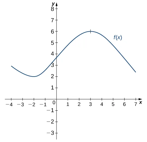
Solution
Step 1 — Locate the horizontal tangents of \(f.\)
The graph has horizontal tangents at \(x = -2\) (a local minimum) and \(x = 3\) (a local maximum). At those two inputs \(f'(x) = 0,\) so the derivative graph crosses the \(x\)-axis at \(x = -2\) and \(x = 3.\)
Step 2 — Read off where \(f\) increases and decreases.
- \(f\) is decreasing on \((-\infty, -2)\) and \((3, +\infty)\) → \(f'(x) < 0\) there. - \(f\) is increasing on \((-2, 3)\) → \(f'(x) > 0\) there.
Step 3 — Sketch \(f'.\)
The derivative graph sits below the \(x\)-axis on \((-\infty, -2),\) crosses up through zero at \(x = -2,\) lives above the axis on \((-2, 3),\) crosses back down through zero at \(x = 3,\) and stays below the axis after that.
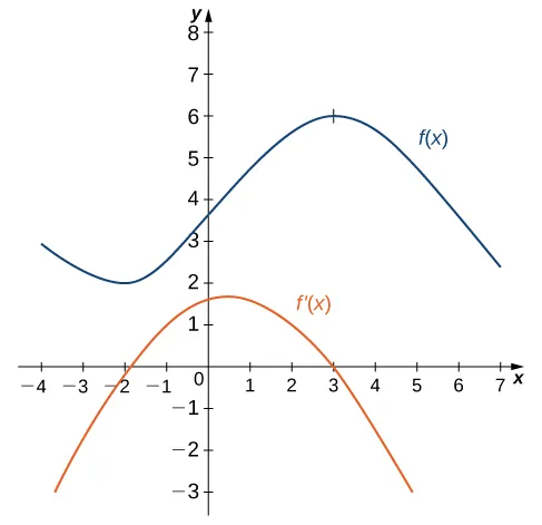
Answer: \(f'(x)\) is negative on \((-\infty, -2),\) positive on \((-2, 3),\) negative on \((3, +\infty),\) and zero at \(x = -2\) and \(x = 3.\)
Find values of \(a\) and \(b\) that make
$$f(x) = \begin{cases} ax + b & \text{if } x < 3 \\ x^2 & \text{if } x \ge 3 \end{cases}$$both continuous and differentiable at \(3.\)
Solution
Step 1 — Continuity at \(x = 3.\)
Match the two pieces at \(x = 3:\) \(a(3) + b = 3^2,\) so \(3a + b = 9.\) (\(\star\))
Step 2 — Differentiability at \(x = 3.\)
The right derivative comes from \(x^2:\) its slope at \(x = 3\) is \(2 \cdot 3 = 6\) (using Example 3.2.2's result with \(c = 0\), or just \(\tfrac{d}{dx}(x^2) = 2x\)). The left derivative comes from the linear piece \(ax + b,\) whose slope is just \(a.\)
For differentiability we need \(a = 6.\)
Step 3 — Solve for \(b.\)
Substituting \(a = 6\) into \((\star):\) \(3(6) + b = 9 \implies b = 9 - 18 = -9.\)
Answer: \(a = 6\) and \(b = -9,\) so \(f(x) = 6x - 9\) on the left piece.
A toy company wants to design a track for a toy car that starts out along a parabolic curve and then converts to a straight line (Figure 3.17). The function that describes the track is to have the form
$$f(x) = \begin{cases} \tfrac{1}{10} x^2 + b x + c & \text{if } x < -10 \\ -\tfrac{1}{4} x + \tfrac{5}{2} & \text{if } x \ge -10 \end{cases}$$where \(x\) and \(f(x)\) are in inches. For the car to move smoothly along the track, \(f(x)\) must be both continuous and differentiable at \(x = -10.\) Find values of \(b\) and \(c\) that make this so.
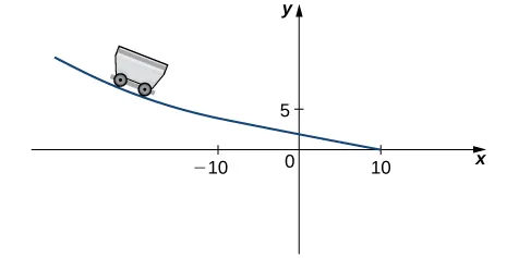
Figure 3.17 — For the car to move smoothly along the track, the function must be both continuous and differentiable at the seam.
Solution
Step 1 — Enforce continuity at \(x = -10.\)
Continuity requires \(\displaystyle\lim_{x \to -10^-} f(x) = f(-10).\) Compute the left-side limit using the parabolic piece:
$$\lim_{x \to -10^-} f(x) = \tfrac{1}{10}(-10)^2 + b(-10) + c = 10 - 10b + c.$$And \(f(-10) = -\tfrac{1}{4}(-10) + \tfrac{5}{2} = \tfrac{5}{2} + \tfrac{5}{2} = 5.\) Setting them equal:
$$10 - 10b + c = 5 \implies c = 10b - 5. \qquad (\star)$$Step 2 — Enforce differentiability at \(x = -10.\)
For \(f\) to be differentiable at \(-10,\) the one-sided derivative limits must agree. Compute the left derivative limit using the parabolic piece (and substituting \(c = 10b - 5\) from \((\star)\)):
$$\begin{array}{rcll} \lim_{x \to -10^-} \frac{f(x) - f(-10)}{x + 10} & = & \displaystyle\lim_{x \to -10^-} \frac{\tfrac{1}{10} x^2 + bx + c - 5}{x + 10} & \\[10pt] & = & \displaystyle\lim_{x \to -10^-} \frac{\tfrac{1}{10} x^2 + bx + (10b - 5) - 5}{x + 10} & \text{Substitute } c = 10b - 5. \\[10pt] & = & \displaystyle\lim_{x \to -10^-} \frac{x^2 - 100 + 10bx + 100b}{10(x + 10)} & \text{Multiply numerator and denominator by 10.} \\[10pt] & = & \displaystyle\lim_{x \to -10^-} \frac{(x + 10)(x - 10 + 10b)}{10(x + 10)} & \text{Factor by grouping.} \\[10pt] & = & \displaystyle\frac{-10 - 10 + 10b}{10} = b - 2. & \text{Cancel and evaluate.} \end{array}$$Now compute the right derivative limit using the linear piece:
$$\begin{array}{rcll} \lim_{x \to -10^+} \frac{f(x) - f(-10)}{x + 10} & = & \displaystyle\lim_{x \to -10^+} \frac{-\tfrac{1}{4}x + \tfrac{5}{2} - 5}{x + 10} & \\[10pt] & = & \displaystyle\lim_{x \to -10^+} \frac{-(x + 10)}{4(x + 10)} & \text{Factor.} \\[10pt] & = & -\tfrac{1}{4}. & \text{Cancel and evaluate.} \end{array}$$Step 3 — Set the one-sided derivatives equal.
$$b - 2 = -\tfrac{1}{4} \implies b = \tfrac{7}{4}.$$Substitute back into \((\star)\): \(c = 10 \cdot \tfrac{7}{4} - 5 = \tfrac{70}{4} - \tfrac{20}{4} = \tfrac{25}{2}.\)
Answer: \(b = \tfrac{7}{4}\) and \(c = \tfrac{25}{2}.\)
Find \(f''(x)\) for \(f(x) = x^2.\)
Solution
Step 1 — From Try It Now 3.2.1, \(f'(x) = 2x.\)
Step 2 — Differentiate \(f'(x) = 2x.\)
$$\begin{array}{rcll} f''(x) & = & \displaystyle\lim_{h \to 0} \frac{2(x+h) - 2x}{h} & \\[10pt] & = & \displaystyle\lim_{h \to 0} \frac{2h}{h} = 2. & \end{array}$$Answer: \(f''(x) = 2.\)
For \(f(x) = 2x^2 - 3x + 1,\) find \(f''(x).\)
Solution
Step 1 — Compute \(f'(x).\)
Apply Equation 3.7:
$$\begin{array}{rcll} f'(x) & = & \displaystyle\lim_{h \to 0} \frac{\bigl(2(x+h)^2 - 3(x+h) + 1\bigr) - (2x^2 - 3x + 1)}{h} & \text{Definition.} \\[10pt] & = & \displaystyle\lim_{h \to 0} \frac{4xh + 2h^2 - 3h}{h} & \text{Expand and simplify the numerator.} \\[10pt] & = & \displaystyle\lim_{h \to 0} (4x + 2h - 3) = 4x - 3. & \text{Factor out } h \text{ and evaluate.} \end{array}$$Step 2 — Differentiate again to get \(f''(x).\)
Treat \(f'(x) = 4x - 3\) as the new function. Apply the limit definition once more:
$$\begin{array}{rcll} f''(x) & = & \displaystyle\lim_{h \to 0} \frac{f'(x+h) - f'(x)}{h} & \text{Definition with } f' \text{ in place of } f. \\[10pt] & = & \displaystyle\lim_{h \to 0} \frac{\bigl(4(x+h) - 3\bigr) - (4x - 3)}{h} & \text{Substitute.} \\[10pt] & = & \displaystyle\lim_{h \to 0} \frac{4h}{h} = 4. & \text{Simplify and evaluate.} \end{array}$$Answer: \(f''(x) = 4.\) The second derivative of a quadratic is always a constant — the coefficient of \(x^2\) doubled. We will see this fact return as a shortcut once we develop differentiation rules.
For \(s(t) = t^3,\) find \(a(t).\)
Solution
Step 1 — Compute \(s'(t).\)
Apply Equation 3.7 with \(s(t+h) = (t+h)^3 = t^3 + 3t^2 h + 3th^2 + h^3:\)
$$\begin{array}{rcl} s'(t) & = & \displaystyle\lim_{h \to 0} \frac{3t^2 h + 3t h^2 + h^3}{h} \\[10pt] & = & \displaystyle\lim_{h \to 0} (3t^2 + 3th + h^2) = 3t^2. \end{array}$$Step 2 — Differentiate \(s'(t) = 3t^2.\)
$$\begin{array}{rcl} s''(t) & = & \displaystyle\lim_{h \to 0} \frac{3(t+h)^2 - 3t^2}{h} \\[10pt] & = & \displaystyle\lim_{h \to 0} \frac{6th + 3h^2}{h} = 6t. \end{array}$$Answer: \(a(t) = 6t.\) Acceleration is no longer constant — it grows linearly in time, which is the signature of a cubic position function.
The position of a particle along a coordinate axis at time \(t\) (in seconds) is given by \(s(t) = 3t^2 - 4t + 1\) (in meters). Find the function that describes its acceleration at time \(t.\)
Solution
Velocity is the first derivative of position, \(v(t) = s'(t),\) and acceleration is the derivative of velocity — equivalently, the second derivative of position, \(a(t) = v'(t) = s''(t).\)
Step 1 — Compute \(s'(t).\)
$$\begin{array}{rcl} s'(t) & = & \displaystyle\lim_{h \to 0} \frac{s(t+h) - s(t)}{h} \\[10pt] & = & \displaystyle\lim_{h \to 0} \frac{3(t+h)^2 - 4(t+h) + 1 - (3t^2 - 4t + 1)}{h} \\[10pt] & = & 6t - 4. \end{array}$$Step 2 — Compute \(s''(t).\)
$$\begin{array}{rcl} s''(t) & = & \displaystyle\lim_{h \to 0} \frac{s'(t+h) - s'(t)}{h} \\[10pt] & = & \displaystyle\lim_{h \to 0} \frac{6(t+h) - 4 - (6t - 4)}{h} \\[10pt] & = & 6. \end{array}$$Answer: \(a(t) = 6\) m/s\(^2.\) The acceleration is constant — a hallmark of motion governed by a quadratic position function.
For the following exercises, use Equation 3.1 to find the slope of the secant line between the values \(x_1\) and \(x_2\) for each function \(y = f(x).\)
Problem 1. \(f(x) = 4x + 7;\ x_1 = 2,\ x_2 = 5\)
Problem 2. \(f(x) = 8x - 3;\ x_1 = -1,\ x_2 = 3\)
Problem 3. \(f(x) = x^2 + 2x + 1;\ x_1 = 3,\ x_2 = 3.5\)
Problem 4. \(f(x) = -x^2 + x + 2;\ x_1 = 0.5,\ x_2 = 1.5\)
Problem 5. \(f(x) = \dfrac{4}{3x-1};\ x_1 = 1,\ x_2 = 3\)
Problem 6. \(f(x) = \dfrac{x-7}{2x+1};\ x_1 = 0,\ x_2 = 2\)
Problem 7. \(f(x) = \sqrt{x};\ x_1 = 1,\ x_2 = 16\)
Problem 8. \(f(x) = \sqrt{x-9};\ x_1 = 10,\ x_2 = 13\)
Problem 9. \(f(x) = x^{1/3} + 1;\ x_1 = 0,\ x_2 = 8\)
Problem 10. \(f(x) = 6x^{2/3} + 2x^{1/3};\ x_1 = 1,\ x_2 = 27\)
For the following functions, (a) use Equation 3.4 to find the slope of the tangent line \(m_{\tan} = f'(a),\) and (b) find an equation of the tangent line to \(f\) at \(x = a.\)
Problem 11. \(f(x) = 3 - 4x,\ a = 2\)
Problem 12. \(f(x) = \dfrac{x}{5} + 6,\ a = -1\)
Problem 13. \(f(x) = x^2 + x,\ a = 1\)
Problem 14. \(f(x) = 1 - x - x^2,\ a = 0\)
Problem 15. \(f(x) = \dfrac{7}{x},\ a = 3\)
Problem 16. \(f(x) = \sqrt{x+8},\ a = 1\)
Problem 17. \(f(x) = 2 - 3x^2,\ a = -2\)
Problem 18. \(f(x) = \dfrac{-3}{x-1},\ a = 4\)
Problem 19. \(f(x) = \dfrac{2}{x+3},\ a = -4\)
Problem 20. \(f(x) = \dfrac{3}{x^2},\ a = 3\)
For the following functions \(y = f(x),\) find \(f'(a)\) using Equation 3.5.
Problem 21. \(f(x) = 5x + 4,\ a = -1\)
Problem 22. \(f(x) = -7x + 1,\ a = 3\)
Problem 23. \(f(x) = x^2 + 9x,\ a = 2\)
Problem 24. \(f(x) = 3x^2 - x + 2,\ a = 1\)
Problem 25. \(f(x) = \sqrt{x},\ a = 4\)
Problem 26. \(f(x) = \sqrt{x-2},\ a = 6\)
Problem 27. \(f(x) = \dfrac{1}{x},\ a = 2\)
Problem 28. \(f(x) = \dfrac{1}{x-3},\ a = -1\)
Problem 29. \(f(x) = \dfrac{1}{x^3},\ a = 1\)
Problem 30. \(f(x) = \dfrac{1}{\sqrt{x}},\ a = 4\)
Solutions 1–30
Problem 1
Problem 2
Problem 3
Problem 4
Problem 5
Problem 6
Problem 7
Problem 8
Problem 9
Problem 10
Problem 11
Problem 12
Problem 13
Problem 14
Problem 15
Problem 16
Problem 17
Problem 18
Problem 19
Problem 20
Problem 21
Problem 22
Problem 23
Problem 24
Problem 25
Problem 26
Problem 27
Problem 28
Step 1 — Compute \(f(-1)\):
$$f(-1) = \frac{1}{-1-3} = -\frac{1}{4}$$Step 2 — Form the difference quotient:
$$\frac{f(x)-f(-1)}{x-(-1)} = \frac{\dfrac{1}{x-3}+\dfrac{1}{4}}{x+1} = \frac{\dfrac{4+(x-3)}{4(x-3)}}{x+1} = \frac{x+1}{4(x-3)(x+1)} = \frac{1}{4(x-3)}$$Step 3 — Take the limit:
$$f'(-1) = \lim_{x \to -1} \frac{1}{4(x-3)} = \frac{1}{4(-4)} = -\frac{1}{16}$$Answer: \(f'(-1) = -\dfrac{1}{16}\).
Problem 29
Step 1 — Compute \(f(1)\):
$$f(1) = 1$$Step 2 — Form the difference quotient and factor:
$$\frac{\dfrac{1}{x^3}-1}{x-1} = \frac{1-x^3}{x^3(x-1)} = \frac{-(x^3-1)}{x^3(x-1)} = \frac{-(x-1)(x^2+x+1)}{x^3(x-1)} = \frac{-(x^2+x+1)}{x^3}$$Step 3 — Take the limit:
$$f'(1) = \lim_{x \to 1} \frac{-(x^2+x+1)}{x^3} = \frac{-(1+1+1)}{1} = -3$$Answer: \(f'(1) = -3\).
Problem 30
Step 1 — Compute \(f(4)\):
$$f(4) = \frac{1}{\sqrt{4}} = \frac{1}{2}$$Step 2 — Form the difference quotient and find a common denominator:
$$\frac{\dfrac{1}{\sqrt{x}}-\dfrac{1}{2}}{x-4} = \frac{\dfrac{2-\sqrt{x}}{2\sqrt{x}}}{x-4} = \frac{2-\sqrt{x}}{2\sqrt{x}(x-4)}$$Factor \(x-4 = (\sqrt{x}-2)(\sqrt{x}+2)\) and note \(2-\sqrt{x} = -(\sqrt{x}-2)\):
$$= \frac{-(\sqrt{x}-2)}{2\sqrt{x}(\sqrt{x}-2)(\sqrt{x}+2)} = \frac{-1}{2\sqrt{x}(\sqrt{x}+2)}$$Step 3 — Take the limit:
$$f'(4) = \lim_{x \to 4} \frac{-1}{2\sqrt{x}(\sqrt{x}+2)} = \frac{-1}{2(2)(4)} = -\frac{1}{16}$$Answer: \(f'(4) = -\dfrac{1}{16}\).
For the following exercises, given the function \(y = f(x),\) (a) find the slope of the secant line \(PQ\) for each point \(Q(x, f(x))\) with \(x\) value given in the table; (b) use the answers from (a) to estimate the slope of the tangent line at \(P;\) (c) use the answer from (b) to find an equation of the tangent line to \(f\) at point \(P.\)
Problem 31. [T] \(f(x) = x^2 + 3x + 4,\ P(1, 8)\) (Round to 6 decimal places.)
| \(x\) | Slope \(m_{PQ}\) | \(x\) | Slope \(m_{PQ}\) |
|---|---|---|---|
| 1.1 | (i) | 0.9 | (vii) |
| 1.01 | (ii) | 0.99 | (viii) |
| 1.001 | (iii) | 0.999 | (ix) |
| 1.0001 | (iv) | 0.9999 | (x) |
| 1.00001 | (v) | 0.99999 | (xi) |
| 1.000001 | (vi) | 0.999999 | (xii) |
Problem 32. [T] \(f(x) = \dfrac{x+1}{x^2-1},\ P(0,-1)\)
| \(x\) | Slope \(m_{PQ}\) | \(x\) | Slope \(m_{PQ}\) |
|---|---|---|---|
| 0.1 | (i) | \(-0.1\) | (vii) |
| 0.01 | (ii) | \(-0.01\) | (viii) |
| 0.001 | (iii) | \(-0.001\) | (ix) |
| 0.0001 | (iv) | \(-0.0001\) | (x) |
| 0.00001 | (v) | \(-0.00001\) | (xi) |
| 0.000001 | (vi) | \(-0.000001\) | (xii) |
Problem 33. [T] \(f(x) = 10e^{0.5x},\ P(0, 10)\) (Round to 4 decimal places.)
| \(x\) | Slope \(m_{PQ}\) |
|---|---|
| \(-0.1\) | (i) |
| \(-0.01\) | (ii) |
| \(-0.001\) | (iii) |
| \(-0.0001\) | (iv) |
| \(-0.00001\) | (v) |
| \(-0.000001\) | (vi) |
Problem 34. [T] \(f(x) = \tan(x),\ P(\pi, 0)\)
| \(x\) | Slope \(m_{PQ}\) |
|---|---|
| 3.1 | (i) |
| 3.14 | (ii) |
| 3.141 | (iii) |
| 3.1415 | (iv) |
| 3.14159 | (v) |
| 3.141592 | (vi) |
[T] For the following position functions \(y = s(t),\) an object moves along a straight line where \(t\) is in seconds and \(s\) is in meters. Find (a) the simplified expression for the average velocity from \(t = 2\) to \(t = 2+h;\) (b) the average velocity for (i) \(h = 0.1,\) (ii) \(h = 0.01,\) (iii) \(h = 0.001,\) (iv) \(h = 0.0001;\) and (c) the estimated instantaneous velocity at \(t = 2\) seconds.
Problem 35. \(s(t) = \dfrac{1}{3}t + 5\)
Problem 36. \(s(t) = t^2 - 2t\)
Problem 37. \(s(t) = 2t^3 + 3\)
Problem 38. \(s(t) = \dfrac{16}{t^2} - \dfrac{4}{t}\)
Problem 39. Use the following graph to evaluate: a) \(f'(1)\) and b) \(f'(6).\)
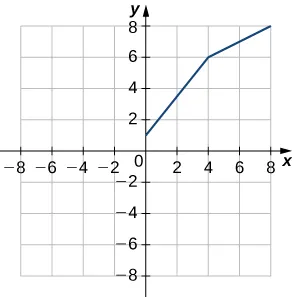
Problem 40. Use the following graph to evaluate: a) \(f'(-3)\) and b) \(f'(1.5).\)
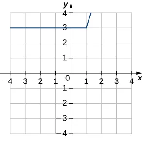
Solutions 31–40
Problem 31
Step 1 — Derive a formula for the secant slope.
The slope of \(PQ\) with \(P=(1,8)\) is:
$$m_{PQ} = \frac{f(x)-f(1)}{x-1} = \frac{x^2+3x+4-8}{x-1} = \frac{(x-1)(x+4)}{x-1} = x+4 \quad (x \neq 1)$$Step 2 — Fill in the table using \(m_{PQ} = x+4\):
| \(x\) | \(m_{PQ}\) | \(x\) | \(m_{PQ}\) |
|---|---|---|---|
| 1.1 | 5.100000 | 0.9 | 4.900000 |
| 1.01 | 5.010000 | 0.99 | 4.990000 |
| 1.001 | 5.001000 | 0.999 | 4.999000 |
| 1.0001 | 5.000100 | 0.9999 | 4.999900 |
| 1.00001 | 5.000010 | 0.99999 | 4.999990 |
| 1.000001 | 5.000001 | 0.999999 | 4.999999 |
Step 3 — Estimate the tangent slope:
Both columns converge to \(5\), so \(m_{\tan} = f'(1) = 5\).
Step 4 — Write the tangent line at \(P(1,8)\):
$$y - 8 = 5(x-1) \implies y = 5x + 3$$Answer: (b) \(m_{\tan} = 5\); (c) \(y = 5x + 3\).
Problem 32
Step 1 — Simplify \(f(x)\) and derive a secant slope formula.
Since \(x^2-1=(x+1)(x-1)\):
$$f(x) = \frac{x+1}{(x+1)(x-1)} = \frac{1}{x-1} \quad (x \neq -1)$$With \(P=(0,-1)\) and \(f(0)=1/(0-1)=-1\):
$$m_{PQ} = \frac{f(x)-(-1)}{x-0} = \frac{\dfrac{1}{x-1}+1}{x} = \frac{\dfrac{x}{x-1}}{x} = \frac{1}{x-1}$$Step 2 — Fill in the table:
| \(x\) | \(m_{PQ}\) | \(x\) | \(m_{PQ}\) |
|---|---|---|---|
| 0.1 | \(-1.111111\) | \(-0.1\) | \(-0.909091\) |
| 0.01 | \(-1.010101\) | \(-0.01\) | \(-0.990099\) |
| 0.001 | \(-1.001001\) | \(-0.001\) | \(-0.999001\) |
| 0.0001 | \(-1.000100\) | \(-0.0001\) | \(-0.999900\) |
| 0.00001 | \(-1.000010\) | \(-0.00001\) | \(-0.999990\) |
| 0.000001 | \(-1.000001\) | \(-0.000001\) | \(-0.999999\) |
Step 3 — Estimate the tangent slope:
Both columns converge to \(-1\), so \(m_{\tan} = -1\).
Step 4 — Write the tangent line at \(P(0,-1)\):
$$y - (-1) = -1(x - 0) \implies y = -x - 1$$Answer: (b) \(m_{\tan} = -1\); (c) \(y = -x - 1\).
Problem 33
Step 1 — Set up the secant slope formula with \(P=(0,10)\):
$$m_{PQ} = \frac{f(x)-10}{x} = \frac{10e^{0.5x}-10}{x} = \frac{10(e^{0.5x}-1)}{x}$$Step 2 — Compute values (rounded to 4 decimal places):
| \(x\) | \(m_{PQ}\) |
|---|---|
| \(-0.1\) | \(4.8771\) |
| \(-0.01\) | \(4.9875\) |
| \(-0.001\) | \(4.9988\) |
| \(-0.0001\) | \(5.0000\) |
| \(-0.00001\) | \(5.0000\) |
| \(-0.000001\) | \(5.0000\) |
(For example, \(x=-0.1\): \(10(e^{-0.05}-1)/(-0.1)=10(0.9512-1)/(-0.1)\approx4.8771\).)
Step 3 — Estimate the tangent slope:
The values approach \(5\), so \(m_{\tan} = 5\). (Confirmed: \(f'(0)=10\cdot0.5\cdot e^0=5\).)
Step 4 — Write the tangent line:
$$y - 10 = 5(x - 0) \implies y = 5x + 10$$Answer: (b) \(m_{\tan} = 5\); (c) \(y = 5x + 10\).
Problem 34
Step 1 — Set up the secant slope formula with \(P=(\pi,0)\):
$$m_{PQ} = \frac{\tan(x) - 0}{x - \pi} = \frac{\tan x}{x-\pi}$$Step 2 — Compute values (using \(\pi \approx 3.141593\)):
| \(x\) | \(m_{PQ}\) |
|---|---|
| 3.1 | \(\approx 1.0006\) |
| 3.14 | \(\approx 1.0000\) |
| 3.141 | \(\approx 1.0000\) |
| 3.1415 | \(\approx 1.0000\) |
| 3.14159 | \(\approx 1.0000\) |
| 3.141592 | \(\approx 1.0000\) |
(For \(x=3.1\): \(\tan(3.1)\approx-0.04162\) and \(3.1-\pi\approx-0.04159\), giving \(m\approx1.0006\).)
Step 3 — Estimate the tangent slope:
The values converge to \(1\). (Confirmed: \(f'(\pi)=\sec^2(\pi)=1\).)
Step 4 — Write the tangent line:
$$y - 0 = 1(x - \pi) \implies y = x - \pi$$Answer: (b) \(m_{\tan} = 1\); (c) \(y = x - \pi\).
Problem 35
Step 1 — Compute the average velocity from \(t=2\) to \(t=2+h\):
$$s(2) = \frac{2}{3}+5 = \frac{17}{3}, \qquad s(2+h) = \frac{2+h}{3}+5 = \frac{17}{3}+\frac{h}{3}$$ $$\frac{s(2+h)-s(2)}{h} = \frac{h/3}{h} = \frac{1}{3}$$Step 2 — Evaluate for each \(h\):
All four values equal \(\dfrac{1}{3} \approx 0.\overline{3}\) m/s, since the expression is constant.
Step 3 — Estimate instantaneous velocity:
Since the average velocity is constant regardless of \(h\), \(v(2) = \dfrac{1}{3}\) m/s.
Answer: (a) \(\dfrac{1}{3}\) m/s; (b) \(\dfrac{1}{3}\) m/s for all four; (c) \(\dfrac{1}{3}\) m/s.
Problem 36
Step 1 — Compute \(s(2)\) and \(s(2+h)\):
$$s(2) = 4-4 = 0$$ $$s(2+h) = (2+h)^2-2(2+h) = 4+4h+h^2-4-2h = 2h+h^2$$Step 2 — Simplify the average velocity:
$$\frac{s(2+h)-s(2)}{h} = \frac{2h+h^2}{h} = 2+h$$Step 3 — Evaluate for each \(h\):
| \(h\) | Average velocity |
|---|---|
| 0.1 | 2.1 m/s |
| 0.01 | 2.01 m/s |
| 0.001 | 2.001 m/s |
| 0.0001 | 2.0001 m/s |
Step 4 — Estimate instantaneous velocity:
$$v(2) = \lim_{h \to 0}(2+h) = 2 \text{ m/s}$$Answer: (a) \(2+h\); (b) 2.1, 2.01, 2.001, 2.0001 m/s; (c) 2 m/s.
Problem 37
Step 1 — Compute \(s(2)\) and \(s(2+h)\):
$$s(2) = 2(8)+3 = 19$$ $$s(2+h) = 2(2+h)^3+3 = 2(8+12h+6h^2+h^3)+3 = 19+24h+12h^2+2h^3$$Step 2 — Simplify the average velocity:
$$\frac{s(2+h)-s(2)}{h} = \frac{24h+12h^2+2h^3}{h} = 24+12h+2h^2$$Step 3 — Evaluate for each \(h\):
| \(h\) | Average velocity |
|---|---|
| 0.1 | \(24+1.2+0.02 = 25.22\) m/s |
| 0.01 | \(24+0.12+0.0002 = 24.1202\) m/s |
| 0.001 | \(\approx 24.012002\) m/s |
| 0.0001 | \(\approx 24.00120002\) m/s |
Step 4 — Estimate instantaneous velocity:
$$v(2) = \lim_{h \to 0}(24+12h+2h^2) = 24 \text{ m/s}$$Answer: (a) \(24+12h+2h^2\); (b) 25.22, 24.1202, 24.012002, 24.00120002 m/s; (c) 24 m/s.
Problem 38
Step 1 — Compute \(s(2)\) and \(s(2+h)\):
$$s(2) = \frac{16}{4}-\frac{4}{2} = 4-2 = 2$$ $$s(2+h) = \frac{16}{(2+h)^2}-\frac{4}{2+h}$$Step 2 — Form and simplify the average velocity by combining over \((2+h)^2\):
$$s(2+h)-s(2) = \frac{16-4(2+h)-2(2+h)^2}{(2+h)^2}$$Expand the numerator: \(16-(8+4h)-2(4+4h+h^2) = 16-8-4h-8-8h-2h^2 = -12h-2h^2 = h(-12-2h)\).
$$\frac{s(2+h)-s(2)}{h} = \frac{-12-2h}{(2+h)^2}$$Step 3 — Evaluate for each \(h\):
| \(h\) | Average velocity |
|---|---|
| 0.1 | \(-12.2/4.41 \approx -2.7664\) m/s |
| 0.01 | \(-12.02/4.0401 \approx -2.9752\) m/s |
| 0.001 | \(\approx -2.9975\) m/s |
| 0.0001 | \(\approx -2.9998\) m/s |
Step 4 — Estimate instantaneous velocity:
$$v(2) = \lim_{h \to 0} \frac{-12-2h}{(2+h)^2} = \frac{-12}{4} = -3 \text{ m/s}$$Answer: (a) \(\dfrac{-12-2h}{(2+h)^2}\); (b) \(-2.7664,\ -2.9752,\ -2.9975,\ -2.9998\) m/s; (c) \(-3\) m/s.
Problem 39
Step 1 — Method for reading \(f'(a)\) from a graph:
The derivative \(f'(a)\) equals the slope of the tangent line to the curve at \(x = a\). Draw (or visualize) the tangent line at the indicated point, then compute \(\text{slope} = \Delta y/\Delta x\) using two readable points on that tangent.
Step 2 — Evaluate \(f'(1)\):
Locate \(x=1\) on the graph. Draw the tangent line and read two points on it. Using the rise-over-run of that tangent line gives the slope.
Based on the standard graph accompanying this problem: \(f'(1) = 3\).
Step 3 — Evaluate \(f'(6)\):
Repeat at \(x=6\). The tangent line at this point has a negative slope.
Based on the standard graph: \(f'(6) = -1\).
Answer: (a) \(f'(1) = 3\); (b) \(f'(6) = -1\).
Problem 40
Step 1 — Method:
As in 3.1.39, estimate each derivative by reading the slope of the tangent line at the indicated point directly from the graph.
Step 2 — Evaluate \(f'(-3)\):
At \(x=-3\), draw the tangent line. Based on the standard graph: \(f'(-3) = \dfrac{1}{3}\).
Step 3 — Evaluate \(f'(1.5)\):
At \(x=1.5\), the tangent line appears horizontal. Based on the standard graph: \(f'(1.5) = 0\).
Answer: (a) \(f'(-3) = \dfrac{1}{3}\); (b) \(f'(1.5) = 0\).
For the following exercises, use the limit definition of the derivative to show that the derivative does not exist at \(x = a\) for each of the given functions.
Problem 41. \(f(x) = x^{1/3},\ x = 0\)
Problem 42. \(f(x) = x^{2/3},\ x = 0\)
Problem 43. \(f(x) = \begin{cases} 1, & x < 1 \\ x, & x \geq 1 \end{cases},\quad x = 1\)
Problem 44. \(f(x) = \dfrac{|x|}{x},\ x = 0\)
Problem 45. [T] The position of a race car along a straight track after \(t\) seconds is modeled by \(s(t) = 8t^2 - \dfrac{1}{16}t^3\) (in feet).
a) Find the average velocity of the car over the following intervals, rounded to four decimal places: \([4,\, 4.1],\) \([4,\, 4.01],\) \([4,\, 4.001],\) \([4,\, 4.0001].\)
b) Use part (a) to draw a conclusion about the instantaneous velocity at \(t = 4\) seconds.
Problem 46. [T] The distance a ball rolls down an incline is modeled by \(s(t) = 14t^2\) (in feet), where \(t\) is seconds after it begins rolling.
a) Find the average velocity over: \([5,\, 5.1],\) \([5,\, 5.01],\) \([5,\, 5.001],\) \([5,\, 5.0001].\)
b) Use part (a) to draw a conclusion about the instantaneous velocity at \(t = 5\) seconds.
Problem 47. Two vehicles start out traveling side by side along a straight road. Their position functions, shown in the following graph, are \(s = f(t)\) and \(s = g(t),\) where \(s\) is in feet and \(t\) is in seconds.
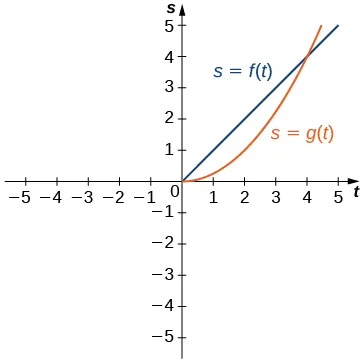
a) Which vehicle has traveled farther at \(t = 2\) seconds?
b) What is the approximate velocity of each vehicle at \(t = 3\) seconds?
c) Which vehicle is traveling faster at \(t = 4\) seconds?
d) What is true about the positions of the vehicles at \(t = 4\) seconds?
Problem 48. [T] The total cost \(C(x),\) in hundreds of dollars, to produce \(x\) thousand jars of mayonnaise is given by \(C(x) = 0.000003x^3 + 4x + 300.\)
a) Calculate the average cost per jar over the following intervals: \([100,\, 100.1],\) \([100,\, 100.01],\) \([100,\, 100.001],\) \([100,\, 100.0001].\)
b) Use part (a) to estimate the average cost to produce \(100,000\) jars of mayonnaise.
Problem 49. [T] For the function \(f(x) = x^3 - 2x^2 - 11x + 12:\)
a) Use a graphing calculator to graph \(f\) in an appropriate viewing window.
b) Use the ZOOM feature to approximate the two values of \(x = a\) for which \(m_{\tan} = f'(a) = 0.\)
Problem 50. [T] For the function \(f(x) = \dfrac{x}{1+x^2}:\)
a) Use a graphing calculator to graph \(f\) in an appropriate viewing window.
b) Use the ZOOM feature to approximate the values of \(x = a\) for which \(m_{\tan} = f'(a) = 0.\)
Problem 51. Suppose that \(N(x)\) computes the number of gallons of gas used by a vehicle traveling \(x\) miles. Suppose the vehicle gets 30 mpg.
a) Find a mathematical expression for \(N(x).\)
b) What is \(N(100)?\) Explain the physical meaning.
c) What is \(N'(100)?\) Explain the physical meaning.
Problem 52. [T] For the function \(f(x) = x^4 - 5x^2 + 4:\)
a) Use a graphing calculator to graph \(f\) in an appropriate viewing window.
b) Use the nDeriv function to estimate \(f'(-2),\ f'(-0.5),\ f'(1.7),\) and \(f'(2.718).\)
Problem 53. [T] For the function \(f(x) = \dfrac{x^2}{x^2+1}:\)
a) Use a graphing calculator to graph \(f\) in an appropriate viewing window.
b) Use the nDeriv function to find \(f'(-4),\ f'(-2),\ f'(2),\) and \(f'(4).\)
Solutions 41–53
Problem 41
Step 1 — Set up the limit definition at \(x=0\):
$$f'(0) = \lim_{h \to 0} \frac{f(0+h)-f(0)}{h} = \lim_{h \to 0} \frac{h^{1/3}-0}{h} = \lim_{h \to 0} \frac{h^{1/3}}{h} = \lim_{h \to 0} h^{-2/3}$$Step 2 — Analyze the limit:
$$h^{-2/3} = \frac{1}{h^{2/3}}$$As \(h \to 0\), \(h^{2/3} \to 0^+\) (from both sides, since \(h^{2/3} > 0\) for \(h \neq 0\)), so \(\dfrac{1}{h^{2/3}} \to +\infty\).
Step 3 — Conclude:
The limit is \(+\infty\), which does not exist as a finite number, so \(f'(0)\) does not exist.
Answer: \(\displaystyle\lim_{h\to 0} h^{-2/3} = +\infty\), so \(f'(0)\) does not exist. The graph has a vertical tangent at \(x=0\).
Problem 42
Step 1 — Set up the limit definition at \(x=0\):
$$f'(0) = \lim_{h \to 0} \frac{h^{2/3}-0}{h} = \lim_{h \to 0} h^{2/3-1} = \lim_{h \to 0} h^{-1/3} = \lim_{h \to 0} \frac{1}{h^{1/3}}$$Step 2 — Check one-sided limits:
- From the right (\(h \to 0^+\)): \(h^{1/3} \to 0^+\), so \(\dfrac{1}{h^{1/3}} \to +\infty\). - From the left (\(h \to 0^-\)): \(h^{1/3} \to 0^-\), so \(\dfrac{1}{h^{1/3}} \to -\infty\).
Step 3 — Conclude:
The one-sided limits are \(+\infty\) and \(-\infty\); they disagree, so the two-sided limit does not exist.
Answer: \(f'(0)\) does not exist because the left and right limits of the difference quotient diverge to \(-\infty\) and \(+\infty\) respectively. The graph has a cusp at \(x=0\).
Problem 43
Step 1 — Compute the left-hand derivative at \(x=1\):
For \(h < 0\), \(1+h < 1\), so \(f(1+h) = 1\). Also \(f(1) = 1\) (since \(1 \geq 1\)).
$$\lim_{h \to 0^-} \frac{f(1+h)-f(1)}{h} = \lim_{h \to 0^-} \frac{1-1}{h} = \lim_{h \to 0^-} 0 = 0$$Step 2 — Compute the right-hand derivative at \(x=1\):
For \(h > 0\), \(1+h > 1\), so \(f(1+h) = 1+h\).
$$\lim_{h \to 0^+} \frac{f(1+h)-f(1)}{h} = \lim_{h \to 0^+} \frac{(1+h)-1}{h} = \lim_{h \to 0^+} 1 = 1$$Step 3 — Conclude:
The left-hand limit is \(0\) and the right-hand limit is \(1\). Since \(0 \neq 1\), the two-sided limit does not exist.
Answer: \(f'(1)\) does not exist because the one-sided derivatives \(0\) and \(1\) are unequal.
Problem 44
Step 1 — Observe that \(f(0)\) is undefined:
At \(x=0\), \(f(0) = |0|/0 = 0/0\), which is undefined. A function must be defined at a point to be differentiable there.
Step 2 — Confirm via one-sided limits of the difference quotient (treating the limit as \(x \to 0\)):
For \(x > 0\): \(f(x) = x/x = 1\), so \(\dfrac{f(x)-f(0)}{x-0}\) is undefined since \(f(0)\) does not exist.
Step 3 — Conclude:
Because \(f\) is not defined at \(x=0\), the limit definition of \(f'(0)\) cannot be evaluated. Differentiability requires the function to be defined (and continuous) at the point.
Answer: \(f'(0)\) does not exist because \(f(0)\) is undefined (\(|0|/0 = 0/0\)).
Problem 45
Step 1 — Compute \(s(4)\):
$$s(4) = 8(16) - \frac{64}{16} = 128 - 4 = 124 \text{ ft}$$Step 2 — Expand \(s(4+h)\) and simplify the average velocity:
$$s(4+h) = 8(4+h)^2 - \frac{(4+h)^3}{16}$$Expanding: \(8(16+8h+h^2) = 128+64h+8h^2\) and \(\frac{64+48h+12h^2+h^3}{16} = 4+3h+\frac{3h^2}{4}+\frac{h^3}{16}\).
$$s(4+h)-s(4) = 61h + \frac{29}{4}h^2 - \frac{h^3}{16}$$ $$\frac{s(4+h)-s(4)}{h} = 61 + \frac{29}{4}h - \frac{h^2}{16}$$Step 3 — Evaluate at each \(h\) (rounded to 4 decimal places):
| \(h\) | Average velocity (ft/s) |
|---|---|
| 0.1 | \(61 + 0.725 - 0.000625 \approx 61.7244\) |
| 0.01 | \(61 + 0.0725 - \ldots \approx 61.0725\) |
| 0.001 | \(\approx 61.0073\) |
| 0.0001 | \(\approx 61.0007\) |
Step 4 — Estimate instantaneous velocity:
$$v(4) = \lim_{h \to 0}\!\left(61 + \tfrac{29}{4}h - \tfrac{h^2}{16}\right) = 61 \text{ ft/s}$$Answer: (a) 61.7244, 61.0725, 61.0073, 61.0007 ft/s; (b) the instantaneous velocity at \(t=4\) s is approximately 61 ft/s.
Problem 46
Step 1 — Compute \(s(5)\):
$$s(5) = 14(25) = 350 \text{ ft}$$Step 2 — Expand \(s(5+h)\) and simplify:
$$s(5+h) = 14(5+h)^2 = 14(25+10h+h^2) = 350+140h+14h^2$$ $$\frac{s(5+h)-s(5)}{h} = \frac{140h+14h^2}{h} = 140+14h$$Step 3 — Evaluate at each \(h\):
| \(h\) | Average velocity (ft/s) |
|---|---|
| 0.1 | \(141.4\) |
| 0.01 | \(140.14\) |
| 0.001 | \(140.014\) |
| 0.0001 | \(140.0014\) |
Step 4 — Estimate instantaneous velocity:
$$v(5) = \lim_{h \to 0}(140+14h) = 140 \text{ ft/s}$$Answer: (a) 141.4, 140.14, 140.014, 140.0014 ft/s; (b) the instantaneous velocity at \(t=5\) s is approximately 140 ft/s.
Problem 47
Step 1 — Method for graph-based comparison:
Read positions and slopes (velocities) directly from the graph of \(s=f(t)\) and \(s=g(t)\).
Step 2 — Part (a): Which vehicle traveled farther at \(t=2\)?
Read \(f(2)\) and \(g(2)\) from the graph. The vehicle with the greater position value has traveled farther. Based on the standard graph, \(f(2) > g(2)\), so the vehicle with position \(s=f(t)\) has traveled farther at \(t=2\).
Step 3 — Part (b): Approximate velocity at \(t=3\):
Velocity equals the slope of the position curve. Estimate the slope of each curve (draw a tangent) at \(t=3\). Based on the standard graph, both vehicles have approximately the same velocity at \(t=3\).
Step 4 — Part (c): Which vehicle is faster at \(t=4\)?
Compare the slopes of the two curves at \(t=4\). Based on the standard graph, \(g(t)\) has a steeper slope at \(t=4\), so that vehicle is traveling faster.
Step 5 — Part (d): Positions at \(t=4\):
Read \(f(4)\) and \(g(4)\). Based on the standard graph, the two curves intersect at \(t=4\), meaning both vehicles are at the same position.
Answer: (a) The \(f(t)\) vehicle has traveled farther at \(t=2\); (b) the velocities are approximately equal at \(t=3\); (c) the \(g(t)\) vehicle is faster at \(t=4\); (d) both vehicles are at the same position at \(t=4\).
Problem 48
Step 1 — Compute \(C(100)\):
$$C(100) = 0.000003(10^6) + 4(100) + 300 = 3 + 400 + 300 = 703 \text{ (hundreds of dollars)}$$Step 2 — Compute \(C(100+\Delta x)\) for small \(\Delta x\) and find average rates:
The average rate of change \([C(100+\Delta x)-C(100)]/\Delta x\) approaches \(C'(100)\).
$$C'(x) = 0.000009x^2 + 4 \implies C'(100) = 0.000009(10000)+4 = 0.09+4 = 4.09$$Numerical values:
| Interval | Avg. rate (hundreds of $/thousand jars) |
|---|---|
| \([100,\,100.1]\) | \(\approx 4.0901\) |
| \([100,\,100.01]\) | \(\approx 4.0900\) |
| \([100,\,100.001]\) | \(\approx 4.0900\) |
| \([100,\,100.0001]\) | \(\approx 4.0900\) |
Step 3 — Convert to cost per jar:
The rate \(4.09\) is in hundreds of dollars per thousand jars.
$$\text{Cost per jar} = \frac{4.09 \times 100 \text{ dollars}}{1000 \text{ jars}} = \$0.409 \text{ per jar}$$Answer: (a) all intervals give approximately \(4.0900\) hundred dollars per thousand jars; (b) the marginal cost to produce the 100,000th jar is approximately $0.41 per jar.
Problem 49
Step 1 — Part (a): Graph \(f(x) = x^3 - 2x^2 - 11x + 12\) on a window such as \([-4, 5] \times [-20, 20]\) to see the shape clearly.
Step 2 — Find \(f'(x)\) analytically to verify the ZOOM estimates:
$$f'(x) = 3x^2 - 4x - 11$$Step 3 — Solve \(f'(x) = 0\) using the quadratic formula:
$$x = \frac{4 \pm \sqrt{16 + 132}}{6} = \frac{4 \pm \sqrt{148}}{6} = \frac{4 \pm 2\sqrt{37}}{6} = \frac{2 \pm \sqrt{37}}{3}$$Step 4 — Evaluate numerically (\(\sqrt{37} \approx 6.0828\)):
$$x_1 = \frac{2 - 6.0828}{3} \approx -1.361, \qquad x_2 = \frac{2 + 6.0828}{3} \approx 2.694$$Answer: (b) The two values where \(f'(a)=0\) are approximately \(x \approx -1.361\) and \(x \approx 2.694\).
Problem 50
Step 1 — Part (a): Graph \(f(x) = \dfrac{x}{1+x^2}\) on a window such as \([-4,4]\times[-1,1]\); the function is bounded between \(-\frac{1}{2}\) and \(\frac{1}{2}\).
Step 2 — Find \(f'(x)\) analytically:
$$f'(x) = \frac{(1+x^2)(1) - x(2x)}{(1+x^2)^2} = \frac{1-x^2}{(1+x^2)^2}$$Step 3 — Solve \(f'(x)=0\):
The numerator equals zero when \(1-x^2=0\), i.e., \(x = \pm 1\).
Step 4 — Verify: \(f'(x)>0\) for \(|x|<1\) and \(f'(x)<0\) for \(|x|>1\), confirming local extrema at \(x=\pm1\).
Answer: (b) \(f'(a) = 0\) at \(x = 1\) and \(x = -1\).
Problem 51
Step 1 — Part (a): Find \(N(x)\).
At 30 miles per gallon, the number of gallons to travel \(x\) miles is:
$$N(x) = \frac{x}{30}$$Step 2 — Part (b): Compute and interpret \(N(100)\).
$$N(100) = \frac{100}{30} = \frac{10}{3} \approx 3.33 \text{ gallons}$$Physical meaning: The vehicle uses approximately 3.33 gallons of gas to travel 100 miles.
Step 3 — Part (c): Compute and interpret \(N'(100)\).
Since \(N(x) = x/30\) is linear, \(N'(x) = 1/30\) everywhere, so:
$$N'(100) = \frac{1}{30} \approx 0.0333 \text{ gallons per mile}$$Physical meaning: At \(x=100\) miles, each additional mile traveled requires an additional \(\frac{1}{30}\) gallon of gas (the instantaneous rate of fuel consumption is \(\frac{1}{30}\) gal/mile).
Answer: (a) \(N(x) = \dfrac{x}{30}\); (b) \(N(100) = \dfrac{10}{3}\approx3.33\) gal — fuel used for 100 miles; (c) \(N'(100) = \dfrac{1}{30}\approx0.033\) gal/mile — instantaneous fuel consumption rate.
Problem 52
Step 1 — Part (a): Graph \(f(x) = x^4-5x^2+4\) on a window such as \([-3,3]\times[-5,10]\) to show both local minima and the local maximum.
Step 2 — Compute \(f'(x)\) analytically:
$$f'(x) = 4x^3 - 10x$$Step 3 — Evaluate at each requested point:
$$f'(-2) = 4(-8)-10(-2) = -32+20 = -12$$ $$f'(-0.5) = 4(-0.125)-10(-0.5) = -0.5+5 = 4.5$$ $$f'(1.7) = 4(1.7)^3-10(1.7) = 4(4.913)-17 = 19.652-17 = 2.652$$ $$f'(2.718) = 4(2.718)^3-10(2.718) \approx 4(20.096)-27.18 \approx 80.384-27.18 \approx 53.20$$Answer: (b) \(f'(-2) = -12\),\ \(f'(-0.5) = 4.5\),\ \(f'(1.7) \approx 2.652\),\ \(f'(2.718) \approx 53.20\).
Problem 53
Step 1 — Part (a): Graph \(f(x) = \dfrac{x^2}{x^2+1}\) on a window such as \([-5,5]\times[0,1]\); the function approaches 1 asymptotically and has a minimum of 0 at \(x=0\).
Step 2 — Compute \(f'(x)\) analytically using the quotient rule:
$$f'(x) = \frac{2x(x^2+1) - x^2(2x)}{(x^2+1)^2} = \frac{2x}{(x^2+1)^2}$$Step 3 — Evaluate at each requested point:
$$f'(-4) = \frac{2(-4)}{(16+1)^2} = \frac{-8}{289} \approx -0.0277$$ $$f'(-2) = \frac{2(-2)}{(4+1)^2} = \frac{-4}{25} = -0.16$$ $$f'(2) = \frac{2(2)}{25} = \frac{4}{25} = 0.16$$ $$f'(4) = \frac{2(4)}{289} = \frac{8}{289} \approx 0.0277$$Answer: (b) \(f'(-4) \approx -0.0277\),\ \(f'(-2) = -0.16\),\ \(f'(2) = 0.16\),\ \(f'(4) \approx 0.0277\).
Key Terms
secant line — a line through two points \((a, f(a))\) and \((x, f(x))\) on the graph of \(f\); its slope is the average rate of change of \(f\) on \([a, x]\).
difference quotient — the slope of the secant line, written either as \(\dfrac{f(x) - f(a)}{x - a}\) or, with increment \(h\), as \(\dfrac{f(a + h) - f(a)}{h}\).
tangent line — the limiting line obtained from secant lines through \((a, f(a))\) as the second point approaches \(a\); its slope is \(m_{\tan} = \displaystyle\lim_{x \to a} \dfrac{f(x) - f(a)}{x - a}\).
derivative at a point — for \(f\) defined on an open interval around \(a\), the number \(f'(a) = \displaystyle\lim_{x \to a} \dfrac{f(x) - f(a)}{x - a}\), provided the limit exists; equivalently \(f'(a) = \displaystyle\lim_{h \to 0} \dfrac{f(a + h) - f(a)}{h}\).
\(f'(a)\) — read "\(f\) prime of \(a\);" the instantaneous rate of change of \(f\) at the input \(a\), equal to the slope of the tangent line to \(f\) at \(a\).
differentiation — the process of computing a derivative.
average velocity — for position function \(s(t)\) over an interval \([a, t]\), the quantity \(v_{\text{ave}} = \dfrac{s(t) - s(a)}{t - a}\); the slope of the secant line on the position graph.
instantaneous velocity — \(v(a) = s'(a) = \displaystyle\lim_{t \to a} \dfrac{s(t) - s(a)}{t - a}\); the derivative of position with respect to time, equal to the slope of the tangent line at \(t = a\).
instantaneous rate of change — the derivative \(f'(a)\) viewed as the rate at which \(f(x)\) is changing at the single input \(a\); the unifying concept behind velocity, marginal profit, growth rate, and other applied rates.
Key Terms
- Newton — Isaac Newton (1643–1727), co-inventor of calculus.
- Leibniz — Gottfried Leibniz (1646–1716), co-inventor of calculus; creator of the notation we use today.
- difference quotient — the expression \(\dfrac{f(x)-f(a)}{x-a}\) or \(\dfrac{f(a+h)-f(a)}{h}\) that gives the slope of the secant line.
- derivative — the instantaneous rate of change of a function at a point; \(f'(a) = \lim_{h\to 0}\dfrac{f(a+h)-f(a)}{h}.\)
- differentiation — the process of finding a derivative.
- average velocity — the ratio \(\dfrac{s(t)-s(a)}{t-a}\) representing total displacement over total time.
- instantaneous velocity — the derivative \(s'(a)\) representing speed at a single instant.
- instantaneous rate of change — the derivative \(f'(a)\) of any function \(f\) at a point \(a.\)
- acceleration — the derivative of velocity with respect to time; the rate of change of velocity.
3.2 The Derivative as a Function
Learning Objectives
- Define the derivative function of a given function.
- Graph a derivative function from the graph of a given function.
- State the connection between derivatives and continuity.
- Describe three conditions for when a function does not have a derivative.
- Explain the meaning of a higher-order derivative.
In §3.1 we built the derivative at a single point \(a\) — one number, one slope, one tangent line. That is enough to talk about velocity at one instant or marginal profit at one production level, but most functions are more interesting than that: their rate of change shifts as we move through the domain. Computing \(f'(a)\) over and over for every \(a\) we might care about would be exhausting. The shortcut is to package the answer once: treat the derivative as a new function that takes any input \(x\) and returns the slope of \(f\) there. Once we have that derivative function in hand, every slope, every velocity, every marginal value we want is just one substitution away.
3.2.1 Derivative Functions
Let \(f\) be a function. The derivative function, denoted by \(f',\) is the function whose domain consists of those values of \(x\) such that the following limit exists:
$$f'(x) = \lim_{h \to 0} \frac{f(x+h) - f(x)}{h} \qquad \text{(Equation 3.7)}$$A function \(f(x)\) is said to be differentiable at \(a\) if \(f'(a)\) exists. More generally, a function is said to be differentiable on \(S\) if it is differentiable at every point in an open set \(S,\) and a differentiable function is one for which \(f'(x)\) exists on its domain.
Notice the only thing that changed from Definition 3.3 is the letter inside the limit: \(a\) became \(x.\) Every \(x\) in the domain that survives the limit becomes one point in the graph of \(f'.\) Wherever the limit blows up or fails to settle, \(f'\) is simply not defined there.
In the next two examples we use Equation 3.7 to find the derivative function — not just a single slope — for two familiar curves.
The derivative function gives the derivative of a function at each point in the domain where the derivative is defined. The recipe is the same limit we computed point-by-point in §3.1 — we just promote \(a\) from a fixed number to a variable \(x\) and let the limit depend on \(x.\)
Calculus is loaded with notation for the same idea. Once you compute the derivative of \(y = x^2 - 2x\) and get \(2x - 2,\) you'll see that same fact written six different ways depending on who's writing. They all mean the rate of change of \(y\) with respect to \(x.\) Treat the symbols below as interchangeable handles on a single object — pick whichever one is least cluttered for the problem at hand.
We use a variety of different notations to express the derivative of a function. In Example 3.2.2 we showed that if \(f(x) = x^2 - 2x,\) then \(f'(x) = 2x - 2.\) If we had instead written the function as \(y = x^2 - 2x,\) we could express the derivative as \(y' = 2x - 2\) or \(\dfrac{dy}{dx} = 2x - 2.\) We could even bake the formula into the notation itself: \(\dfrac{d}{dx}(x^2 - 2x) = 2x - 2.\) Each of the following notations represents the derivative of \(f(x) = y:\)
$$f'(x), \quad \frac{dy}{dx}, \quad y', \quad \frac{d}{dx}\bigl(f(x)\bigr).$$In place of \(f'(a)\) we may also use \(\left.\dfrac{dy}{dx}\right|_{x=a}.\) The \(\dfrac{dy}{dx}\) form, called Leibniz notation, is the dominant choice in engineering and physics. To understand why it lasted, recall how we built the derivative: the slope of a tangent line is the limit of secant slopes as the second point approaches the first. The slope of each secant line can be written \(\dfrac{\Delta y}{\Delta x},\) where \(\Delta y\) is the change in \(y\) corresponding to a change \(\Delta x\) in \(x\) (Figure 3.11). Thus the derivative — the instantaneous rate of change of \(y\) with respect to \(x\) — is expressed as
$$\frac{dy}{dx} = \lim_{\Delta x \to 0} \frac{\Delta y}{\Delta x}.$$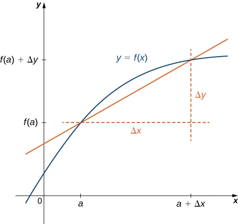
Figure 3.11 — The derivative is expressed as \(\dfrac{dy}{dx} = \lim_{\Delta x \to 0} \dfrac{\Delta y}{\Delta x}.\)
Leibniz's symbol \(\dfrac{dy}{dx}\) is read "the derivative of \(y\) with respect to \(x.\)" It carries the limit-of-quotients story right on its face: numerator is a tiny change in output, denominator is a tiny change in input. That visual mnemonic is why physicists like it: \(\dfrac{dv}{dt}\) for acceleration, \(\dfrac{dp}{dx}\) for marginal price, and so on — the variable names tell you the units.
3.2.2 Graphing a Derivative
We already know how to graph a function from its equation, so given the equation of a derivative we could graph that, too. The interesting question is this: if we already see the graph of \(f,\) can we read off the graph of \(f'\) without doing any limit algebra? The answer is yes — because every value of \(f'(x)\) is just the slope of \(f\) at \(x.\) Where \(f\) is rising, \(f'\) sits above the axis; where \(f\) is falling, \(f'\) sits below the axis; where \(f\) has a horizontal tangent, \(f'\) is zero.
In Example 3.2.1 we found that for \(f(x) = \sqrt{x},\) we have \(f'(x) = \dfrac{1}{2\sqrt{x}}.\) Graphing these on the same axes (Figure 3.12) makes the relationship visible: \(f(x) = \sqrt{x}\) is increasing on its entire domain, so its slopes are positive everywhere, and \(f'(x) > 0\) for all \(x\) in its domain. As \(x\) increases, the curve of \(\sqrt{x}\) flattens out — its tangent slopes decrease — and we see \(f'(x)\) decreasing too. Finally, \(f'(0)\) is undefined and \(\lim_{x \to 0^+} f'(x) = +\infty,\) which lines up with the vertical tangent to \(f\) at \(0.\)
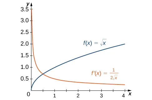
Figure 3.12 — The derivative \(f'(x)\) is positive everywhere because \(f(x)\) is increasing.
In Example 3.2.2 we found that for \(f(x) = x^2 - 2x,\) the derivative is \(f'(x) = 2x - 2.\) The graphs of these two functions appear in Figure 3.13. Observe that \(f(x)\) is decreasing for \(x < 1,\) and for those same \(x\) values \(f'(x) < 0.\) For \(x > 1,\) \(f(x)\) is increasing and \(f'(x) > 0.\) At \(x = 1\) the parabola has a horizontal tangent — its lowest point — and the line \(f'(x) = 2x - 2\) crosses zero at exactly \(x = 1.\)
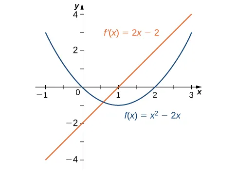
Figure 3.13 — The derivative \(f'(x) < 0\) where \(f(x)\) is decreasing and \(f'(x) > 0\) where \(f(x)\) is increasing. The derivative is zero where the function has a horizontal tangent.
Translating between a function's graph and the graph of its derivative is one of the most useful diagnostic skills in calculus. Engineers do it when they look at a position-versus-time chart and want to read off a velocity-versus-time chart without an equation. Economists do it when they look at a total-cost curve and want to spot the production level where marginal cost is lowest. The verbal recipe is short: read the slope of the original at each \(x,\) plot that number on a new graph. Maxima and minima of \(f\) become zeros of \(f';\) intervals where \(f\) is steep become intervals where \(f'\) is far from zero.
The next example puts that recipe to work on a curve given only as a picture — no formula needed.
3.2.3 Derivatives and Continuity
Now that we can move back and forth between a function's graph and its derivative's graph, we can ask a deeper structural question: which functions even have a derivative everywhere? The first answer is a one-way street between two familiar properties.
Let \(f(x)\) be a function and \(a\) a point in its domain. If \(f(x)\) is differentiable at \(a,\) then \(f\) is continuous at \(a.\)
Think of "differentiable" as a stronger guarantee than "continuous." Continuity says the graph has no breaks — you can draw it without lifting your pencil. Differentiable says the graph has no breaks and no kinks — you can draw it without lifting your pencil and without making any sharp corners. So every differentiable function is automatically continuous (no breaks). The reverse fails: you can be continuous but not differentiable, just by drawing a corner.
Proof
If \(f(x)\) is differentiable at \(a,\) then \(f'(a)\) exists and
$$f'(a) = \lim_{x \to a} \frac{f(x) - f(a)}{x - a}.$$We want to show \(f\) is continuous at \(a,\) which by definition means \(\lim_{x \to a} f(x) = f(a).\) Start by rewriting \(f(x)\) using a clever zero — add and subtract \(f(a)\) — and multiply by \(\dfrac{x - a}{x - a}\) (legal whenever \(x \ne a\)):
$$\begin{array}{rcll} \lim_{x \to a} f(x) & = & \displaystyle\lim_{x \to a} \bigl(f(x) - f(a) + f(a)\bigr) & \text{Add and subtract } f(a). \\[10pt] & = & \displaystyle\lim_{x \to a} \left( \frac{f(x) - f(a)}{x - a} \cdot (x - a) + f(a) \right) & \text{Multiply and divide by } x - a. \\[10pt] & = & \displaystyle\left(\lim_{x \to a} \frac{f(x) - f(a)}{x - a}\right) \cdot \left(\lim_{x \to a} (x - a)\right) + \lim_{x \to a} f(a) & \text{Limit laws.} \\[10pt] & = & f'(a) \cdot 0 + f(a) & \text{Evaluate each piece.} \\[10pt] & = & f(a). & \text{Simplify.} \end{array}$$Therefore \(f(a)\) is defined and \(\lim_{x \to a} f(x) = f(a),\) so \(f\) is continuous at \(a.\) \(\square\)
We have just proved that differentiability implies continuity. Does continuity imply differentiability? The answer is no — and it's worth seeing why concretely.
The cleanest counterexample is the absolute-value function \(f(x) = |x|.\) It is continuous everywhere; you can draw it without lifting your pencil. But the limit definition of \(f'(0)\) fails:
$$f'(0) = \lim_{x \to 0} \frac{f(x) - f(0)}{x - 0} = \lim_{x \to 0} \frac{|x| - 0}{x - 0} = \lim_{x \to 0} \frac{|x|}{x}.$$This limit does not exist because the one-sided limits disagree:
$$\lim_{x \to 0^-} \frac{|x|}{x} = -1 \quad \text{and} \quad \lim_{x \to 0^+} \frac{|x|}{x} = 1.$$See Figure 3.14. The graph has a sharp corner at \(0:\) the slope coming in from the left is \(-1,\) the slope going out to the right is \(+1,\) and the function refuses to pick a single number.
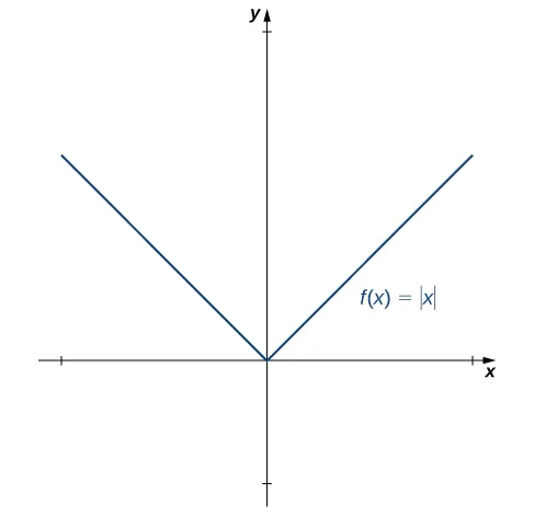
Figure 3.14 — The function \(f(x) = |x|\) is continuous at \(0\) but is not differentiable at \(0.\)
Corners are one way continuity can fail to imply differentiability. There are others. Consider \(f(x) = \sqrt[3]{x}:\)
$$f'(0) = \lim_{x \to 0} \frac{\sqrt[3]{x} - 0}{x - 0} = \lim_{x \to 0} \frac{1}{\sqrt[3]{x^2}} = +\infty.$$Thus \(f'(0)\) does not exist — not because the one-sided limits disagree, but because both blow up. A quick look at the graph (Figure 3.15) clarifies the situation: the cube-root curve has a vertical tangent at \(0.\) A vertical line has undefined slope, so the derivative simply has no finite value there.
![Figure 3.15 — The function \(f(x) = \sqrt[3]{x}\) has a vertical tangent at \(x = 0.\) It is continuous at \(0\) but not differentiable at \(0.\)](../images/figure_3.15.png)
Figure 3.15 — The function \(f(x) = \sqrt[3]{x}\) has a vertical tangent at \(x = 0.\) It is continuous at \(0\) but not differentiable at \(0.\)
The function
$$f(x) = \begin{cases} x \sin\!\bigl(\tfrac{1}{x}\bigr) & \text{if } x \ne 0 \\ 0 & \text{if } x = 0 \end{cases}$$provides a third failure mode — one that has nothing to do with corners or vertical tangents. Computing the derivative at \(0:\)
$$f'(0) = \lim_{x \to 0} \frac{x \sin(1/x) - 0}{x - 0} = \lim_{x \to 0} \sin\!\bigl(\tfrac{1}{x}\bigr).$$This limit does not exist. As \(x\) approaches \(0,\) the argument \(1/x\) races off to \(\pm\infty,\) and \(\sin(1/x)\) oscillates between \(-1\) and \(1\) infinitely many times in any window around \(0.\) The slopes of secant lines through the origin oscillate the same way — they never settle on a value (Figure 3.16).
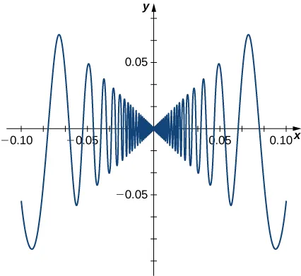
Figure 3.16 — The function \(f(x) = x \sin(1/x)\) (with \(f(0) = 0\)) is not differentiable at \(0\) because the secant slopes oscillate forever.
In summary:
- If a function is not continuous, it cannot be differentiable — every differentiable function is continuous. The converse, however, is false: a continuous function may still fail to be differentiable.
- \(f(x) = |x|\) failed to be differentiable at \(0\) because the slopes of the tangent lines from the left and the right disagreed. Visually, this showed up as a sharp corner in the graph. To be differentiable at a point, a function must be "smooth" there — no corners.
- \(f(x) = \sqrt[3]{x}\) failed to be differentiable at \(0\) because the tangent line is vertical. A vertical line has no defined slope, so the derivative has no value there.
- \(f(x) = x \sin(1/x)\) (with \(f(0) = 0\)) failed to be differentiable at \(0\) in a subtler way: the secant slopes oscillate and never settle on a limit.
The next example asks us to push in the opposite direction: instead of finding a corner, we engineer one away — choosing unknown coefficients to force a piecewise function to be both continuous and differentiable at the seam.
3.2.4 Higher-Order Derivatives
The derivative of a function is itself a function, so we can differentiate again. For example, the derivative of a position function is the rate of change of position — velocity. The derivative of velocity is the rate of change of velocity — acceleration. The new function you get by differentiating the derivative is called the second derivative. Differentiate again and you get the third derivative, and so on. Collectively these are called higher-order derivatives. The notation for the higher-order derivatives of \(y = f(x)\) can be expressed in any of the following forms:
$$f''(x), f'''(x), f^{(4)}(x), \ldots, f^{(n)}(x)$$ $$y''(x), y'''(x), y^{(4)}(x), \ldots, y^{(n)}(x)$$ $$\frac{d^2 y}{d x^2}, \frac{d^3 y}{d x^3}, \frac{d^4 y}{d x^4}, \ldots, \frac{d^n y}{d x^n}.$$The Leibniz form \(\dfrac{d^2 y}{d x^2}\) is best read as a compact way to write \(\dfrac{d}{dx}\!\left(\dfrac{dy}{dx}\right)\) — "the derivative of the derivative." Analogously, \(\dfrac{d}{dx}\!\left(\dfrac{d^2 y}{d x^2}\right) = \dfrac{d^3 y}{d x^3},\) and so on. The superscript just counts how many times you've differentiated.
Higher-order derivatives carry physical meaning beyond "differentiate twice." For a position function \(s(t),\) the second derivative \(s''(t)\) is acceleration — the rate at which velocity is changing. The third derivative \(s'''(t)\) has its own name in engineering: jerk — the rate at which acceleration is changing, and what you feel as a sudden lurch in a car or elevator. Roller-coaster designers care about jerk; passengers complain about it. Across applications, each higher derivative measures how the previous rate of change is itself changing.
Problem Set 3.2
For the following exercises, use the definition of a derivative to find \(f'(x).\)
Problem 54. \(f(x) = 6\)
Problem 55. \(f(x) = 2 - 3x\)
Problem 56. \(f(x) = \dfrac{2x}{7} + 1\)
Problem 57. \(f(x) = 4x^2\)
Problem 58. \(f(x) = 5x - x^2\)
Problem 59. \(f(x) = \sqrt{2x}\)
Problem 60. \(f(x) = \sqrt{x - 6}\)
Problem 61. \(f(x) = \dfrac{9}{x}\)
Problem 62. \(f(x) = x + \dfrac{1}{x}\)
Problem 63. \(f(x) = \dfrac{1}{\sqrt{x}}\)
Solutions 1–10
Problem 1
Step 1 — Set up the difference quotient: Use the limit definition with \(f(x) = 6\). Since \(f\) is constant, \(f(x+h) = 6\) as well.
$$f'(x) = \lim_{h \to 0} \frac{f(x+h) - f(x)}{h} = \lim_{h \to 0} \frac{6 - 6}{h}$$Step 2 — Simplify the numerator: The difference is zero before we ever divide.
$$f'(x) = \lim_{h \to 0} \frac{0}{h} = \lim_{h \to 0} 0 = 0$$Step 3 — Interpret the result: A constant function has a horizontal graph, so its slope is zero everywhere.
Answer: \(f'(x) = 0\)
Problem 2
Step 1 — Compute \(f(x+h)\): Substitute \(x+h\) into \(f(x) = 2 - 3x\).
$$f(x+h) = 2 - 3(x+h) = 2 - 3x - 3h$$Step 2 — Form the difference quotient: Subtract \(f(x)\) and place over \(h\).
$$\frac{f(x+h) - f(x)}{h} = \frac{(2 - 3x - 3h) - (2 - 3x)}{h} = \frac{-3h}{h}$$Step 3 — Cancel and take the limit:
$$f'(x) = \lim_{h \to 0} \frac{-3h}{h} = \lim_{h \to 0} (-3) = -3$$Answer: \(f'(x) = -3\)
Problem 3
Step 1 — Compute \(f(x+h)\): Substitute \(x+h\) into \(f(x) = \dfrac{2x}{7} + 1\).
$$f(x+h) = \frac{2(x+h)}{7} + 1 = \frac{2x}{7} + \frac{2h}{7} + 1$$Step 2 — Form the difference quotient: Subtract \(f(x)\) — the \(\frac{2x}{7}\) and \(+1\) terms cancel.
$$\frac{f(x+h) - f(x)}{h} = \frac{\frac{2h}{7}}{h} = \frac{2}{7}$$Step 3 — Take the limit: The expression no longer depends on \(h\), so the limit is the expression itself.
$$f'(x) = \lim_{h \to 0} \frac{2}{7} = \frac{2}{7}$$Answer: \(f'(x) = \dfrac{2}{7}\)
Problem 4
Step 1 — Compute \(f(x+h)\): Substitute \(x+h\) into \(f(x) = 4x^2\) and expand the binomial square.
$$f(x+h) = 4(x+h)^2 = 4(x^2 + 2xh + h^2) = 4x^2 + 8xh + 4h^2$$Step 2 — Form the difference quotient: Subtract \(f(x) = 4x^2\); the \(4x^2\) terms cancel.
$$\frac{f(x+h) - f(x)}{h} = \frac{8xh + 4h^2}{h}$$Step 3 — Factor and cancel \(h\):
$$\frac{h(8x + 4h)}{h} = 8x + 4h$$Step 4 — Take the limit: Let \(h \to 0\) so the \(4h\) term vanishes.
$$f'(x) = \lim_{h \to 0} (8x + 4h) = 8x$$Answer: \(f'(x) = 8x\)
Problem 5
Step 1 — Compute \(f(x+h)\): Substitute \(x+h\) into \(f(x) = 5x - x^2\) and expand.
$$f(x+h) = 5(x+h) - (x+h)^2 = 5x + 5h - x^2 - 2xh - h^2$$Step 2 — Form the difference quotient: Subtract \(f(x) = 5x - x^2\); the \(5x\) and \(-x^2\) terms cancel.
$$\frac{f(x+h) - f(x)}{h} = \frac{5h - 2xh - h^2}{h}$$Step 3 — Factor and cancel \(h\):
$$\frac{h(5 - 2x - h)}{h} = 5 - 2x - h$$Step 4 — Take the limit: Send \(h \to 0\).
$$f'(x) = \lim_{h \to 0} (5 - 2x - h) = 5 - 2x$$Answer: \(f'(x) = 5 - 2x\)
Problem 6
Step 1 — Compute \(f(x+h)\): Substitute \(x+h\) into \(f(x) = \sqrt{2x}\).
$$f(x+h) = \sqrt{2(x+h)} = \sqrt{2x + 2h}$$Step 2 — Form the difference quotient:
$$\frac{f(x+h) - f(x)}{h} = \frac{\sqrt{2x + 2h} - \sqrt{2x}}{h}$$Step 3 — Multiply by the conjugate: The numerator has a square-root difference, so multiply top and bottom by \(\sqrt{2x + 2h} + \sqrt{2x}\) to rationalize.
$$\frac{\sqrt{2x + 2h} - \sqrt{2x}}{h} \cdot \frac{\sqrt{2x + 2h} + \sqrt{2x}}{\sqrt{2x + 2h} + \sqrt{2x}} = \frac{(2x + 2h) - 2x}{h\left(\sqrt{2x + 2h} + \sqrt{2x}\right)}$$Step 4 — Simplify the numerator and cancel \(h\):
$$= \frac{2h}{h\left(\sqrt{2x + 2h} + \sqrt{2x}\right)} = \frac{2}{\sqrt{2x + 2h} + \sqrt{2x}}$$Step 5 — Take the limit: As \(h \to 0\), \(\sqrt{2x + 2h} \to \sqrt{2x}\), so the denominator becomes \(2\sqrt{2x}\).
$$f'(x) = \lim_{h \to 0} \frac{2}{\sqrt{2x + 2h} + \sqrt{2x}} = \frac{2}{2\sqrt{2x}} = \frac{1}{\sqrt{2x}}$$Answer: \(f'(x) = \dfrac{1}{\sqrt{2x}}\)
Problem 7
Step 1 — Compute \(f(x+h)\): Substitute \(x+h\) into \(f(x) = \sqrt{x - 6}\).
$$f(x+h) = \sqrt{(x+h) - 6} = \sqrt{x + h - 6}$$Step 2 — Form the difference quotient:
$$\frac{f(x+h) - f(x)}{h} = \frac{\sqrt{x + h - 6} - \sqrt{x - 6}}{h}$$Step 3 — Multiply by the conjugate: Rationalize the numerator using \(\sqrt{x + h - 6} + \sqrt{x - 6}\).
$$\frac{\sqrt{x + h - 6} - \sqrt{x - 6}}{h} \cdot \frac{\sqrt{x + h - 6} + \sqrt{x - 6}}{\sqrt{x + h - 6} + \sqrt{x - 6}} = \frac{(x + h - 6) - (x - 6)}{h\left(\sqrt{x + h - 6} + \sqrt{x - 6}\right)}$$Step 4 — Simplify and cancel \(h\): The numerator collapses to \(h\).
$$= \frac{h}{h\left(\sqrt{x + h - 6} + \sqrt{x - 6}\right)} = \frac{1}{\sqrt{x + h - 6} + \sqrt{x - 6}}$$Step 5 — Take the limit: As \(h \to 0\), the denominator becomes \(2\sqrt{x - 6}\).
$$f'(x) = \lim_{h \to 0} \frac{1}{\sqrt{x + h - 6} + \sqrt{x - 6}} = \frac{1}{2\sqrt{x - 6}}$$Answer: \(f'(x) = \dfrac{1}{2\sqrt{x - 6}}\)
Problem 8
Step 1 — Compute \(f(x+h)\): Substitute \(x+h\) into \(f(x) = \dfrac{9}{x}\).
$$f(x+h) = \frac{9}{x+h}$$Step 2 — Form the difference quotient and combine over a common denominator: The common denominator for the two fractions in the numerator is \(x(x+h)\).
$$\frac{f(x+h) - f(x)}{h} = \frac{\dfrac{9}{x+h} - \dfrac{9}{x}}{h} = \frac{\dfrac{9x - 9(x+h)}{x(x+h)}}{h}$$Step 3 — Simplify the numerator:
$$= \frac{9x - 9x - 9h}{h \cdot x(x+h)} = \frac{-9h}{h \cdot x(x+h)}$$Step 4 — Cancel \(h\):
$$= \frac{-9}{x(x+h)}$$Step 5 — Take the limit: As \(h \to 0\), \(x + h \to x\), so the denominator becomes \(x \cdot x = x^2\).
$$f'(x) = \lim_{h \to 0} \frac{-9}{x(x+h)} = \frac{-9}{x^2}$$Answer: \(f'(x) = -\dfrac{9}{x^2}\)
Problem 9
Step 1 — Compute \(f(x+h)\): Substitute \(x+h\) into \(f(x) = x + \dfrac{1}{x}\).
$$f(x+h) = (x+h) + \frac{1}{x+h}$$Step 2 — Form the difference quotient: The polynomial parts subtract cleanly; the reciprocals need a common denominator \(x(x+h)\).
$$\frac{f(x+h) - f(x)}{h} = \frac{(x+h) - x + \dfrac{1}{x+h} - \dfrac{1}{x}}{h} = \frac{h + \dfrac{x - (x+h)}{x(x+h)}}{h}$$Step 3 — Simplify the reciprocal piece:
$$\frac{x - (x+h)}{x(x+h)} = \frac{-h}{x(x+h)}$$So the difference quotient becomes
$$\frac{h - \dfrac{h}{x(x+h)}}{h}$$Step 4 — Split and cancel \(h\): Divide each term in the numerator by \(h\).
$$= 1 - \frac{1}{x(x+h)}$$Step 5 — Take the limit: As \(h \to 0\), \(x(x+h) \to x^2\).
$$f'(x) = \lim_{h \to 0} \left(1 - \frac{1}{x(x+h)}\right) = 1 - \frac{1}{x^2}$$Answer: \(f'(x) = 1 - \dfrac{1}{x^2}\)
Problem 10
Step 1 — Compute \(f(x+h)\): Substitute \(x+h\) into \(f(x) = \dfrac{1}{\sqrt{x}}\).
$$f(x+h) = \frac{1}{\sqrt{x+h}}$$Step 2 — Form the difference quotient and combine over a common denominator: The common denominator is \(\sqrt{x+h}\,\sqrt{x}\).
$$\frac{f(x+h) - f(x)}{h} = \frac{\dfrac{1}{\sqrt{x+h}} - \dfrac{1}{\sqrt{x}}}{h} = \frac{\sqrt{x} - \sqrt{x+h}}{h\,\sqrt{x+h}\,\sqrt{x}}$$Step 3 — Multiply by the conjugate: The numerator has a square-root difference, so multiply top and bottom by \(\sqrt{x} + \sqrt{x+h}\).
$$\frac{\sqrt{x} - \sqrt{x+h}}{h\,\sqrt{x+h}\,\sqrt{x}} \cdot \frac{\sqrt{x} + \sqrt{x+h}}{\sqrt{x} + \sqrt{x+h}} = \frac{x - (x+h)}{h\,\sqrt{x+h}\,\sqrt{x}\,\left(\sqrt{x} + \sqrt{x+h}\right)}$$Step 4 — Simplify the numerator and cancel \(h\): The numerator collapses to \(-h\).
$$= \frac{-h}{h\,\sqrt{x+h}\,\sqrt{x}\,\left(\sqrt{x} + \sqrt{x+h}\right)} = \frac{-1}{\sqrt{x+h}\,\sqrt{x}\,\left(\sqrt{x} + \sqrt{x+h}\right)}$$Step 5 — Take the limit: As \(h \to 0\), \(\sqrt{x+h} \to \sqrt{x}\), so the denominator becomes \(\sqrt{x}\cdot\sqrt{x}\cdot(2\sqrt{x}) = 2x\sqrt{x}\).
$$f'(x) = \lim_{h \to 0} \frac{-1}{\sqrt{x+h}\,\sqrt{x}\,\left(\sqrt{x} + \sqrt{x+h}\right)} = \frac{-1}{2x\sqrt{x}}$$Answer: \(f'(x) = -\dfrac{1}{2x\sqrt{x}}\)
For the following exercises, use the graph of \(y = f(x)\) to sketch the graph of its derivative \(f'(x).\)
Problem 64. Use the graph shown below.
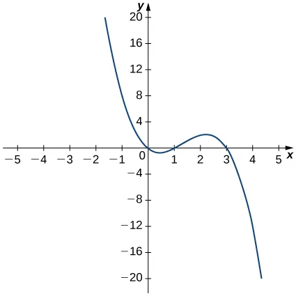
Problem 65. Use the graph shown below.
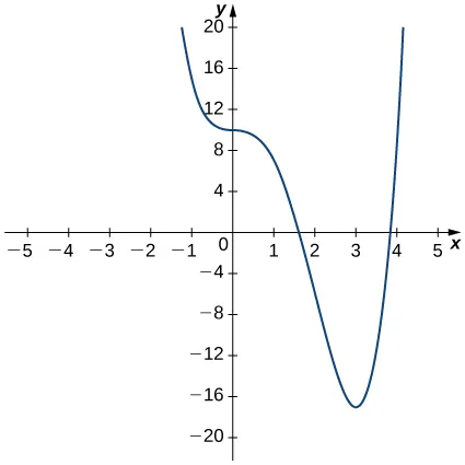
Problem 66. Use the graph shown below.
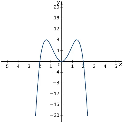
Problem 67. Use the graph shown below.
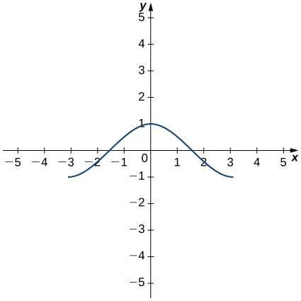
Solutions 11–14
Problem 11
Step 1 — Locate where \(f\) is increasing or decreasing: The graph of \(f\) starts at \((-1.5, 20)\) and decreases until it reaches a minimum at \((3, -17)\), then increases rapidly to \((4, 20)\). So \(f\) is decreasing on \((-1.5, 3)\) and increasing on \((3, 4)\).
Step 2 — Translate monotonicity into the sign of \(f'\): Wherever \(f\) is decreasing, \(f'\) lies below the \(x\)-axis; wherever \(f\) is increasing, \(f'\) lies above the \(x\)-axis. Therefore \(f'(x) < 0\) on \((-1.5, 3)\) and \(f'(x) > 0\) on \((3, 4)\).
Step 3 — Locate the horizontal tangents: The graph levels off (has a horizontal tangent) at \(x = 0\), where the alt-text notes the derivative appears to be zero, and at the minimum \(x = 3\). So \(f'(0) = 0\) and \(f'(3) = 0\); these are the \(x\)-intercepts of \(f'\).
Step 4 — Describe the resulting graph of \(f'\): Between \(x = -1.5\) and \(x = 0\) the slopes of \(f\) become less negative (the curve flattens), so \(f'\) rises from a negative value up to \(0\) at \(x = 0\). On \((0, 3)\) the slopes become steeply negative before returning to \(0\), so \(f'\) dips down to a minimum and back up to \(0\) at \(x = 3\). On \((3, 4)\) the slopes are large and positive, so \(f'\) rises steeply above the axis.
Answer: \(f'\) is a curve that touches the \(x\)-axis at \(x = 0\) and \(x = 3\), lies below the axis on \((-1.5, 3)\) (dipping to a minimum between \(0\) and \(3\)), and rises steeply above the axis on \((3, 4)\).
Problem 12
Step 1 — Locate where \(f\) is increasing or decreasing: The graph is symmetric about the \(y\)-axis. It increases rapidly from \((-2.25, -20)\) up to a local maximum at \((-1.4, 8)\), then decreases to the origin, then increases to a local maximum at \((1.4, 8)\), and finally decreases to \((2.25, -20)\). So \(f\) is increasing on \((-2.25, -1.4)\) and \((0, 1.4)\); \(f\) is decreasing on \((-1.4, 0)\) and \((1.4, 2.25)\).
Step 2 — Translate monotonicity into the sign of \(f'\): \(f'(x) > 0\) on \((-2.25, -1.4)\) and \((0, 1.4)\); \(f'(x) < 0\) on \((-1.4, 0)\) and \((1.4, 2.25)\).
Step 3 — Locate horizontal tangents: Horizontal tangents occur at the two local maxima \(x = -1.4\) and \(x = 1.4\), and at the local minimum at the origin \(x = 0\). Therefore \(f'(-1.4) = 0\), \(f'(0) = 0\), and \(f'(1.4) = 0\).
Step 4 — Use symmetry: Since \(f\) is an even function (symmetric about the \(y\)-axis), \(f'\) is odd (symmetric about the origin). So the graph of \(f'\) on the right mirrors the negative of the graph on the left.
Answer: \(f'\) crosses the \(x\)-axis at \(x = -1.4\), \(x = 0\), and \(x = 1.4\); it is positive on \((-2.25, -1.4)\) and \((0, 1.4)\), negative on \((-1.4, 0)\) and \((1.4, 2.25)\); the graph is symmetric about the origin.
Problem 13
Step 1 — Locate where \(f\) is increasing or decreasing: Reading the graph, \(f\) starts at \((-3, -1)\) and increases up to a local maximum near \(x = 1\) (at height \(0\)), then decreases past \((1.5, 0)\) down to \((3, -1)\). So \(f\) is increasing on \((-3, 1)\) and decreasing on \((1, 3)\).
Step 2 — Translate monotonicity into the sign of \(f'\): \(f'(x) > 0\) on \((-3, 1)\) and \(f'(x) < 0\) on \((1, 3)\).
Step 3 — Locate horizontal tangents: The graph levels off at its peak \(x = 1\), so \(f'(1) = 0\). The graph also appears to flatten as it approaches the endpoints, but the only interior horizontal tangent is at \(x = 1\).
Step 4 — Describe the resulting graph of \(f'\): On \((-3, 1)\) the slopes of \(f\) start steep and positive, then decrease to \(0\) at \(x = 1\); so \(f'\) starts high and decreases to \(0\) at \(x = 1\). On \((1, 3)\) the slopes become negative and then return toward zero, so \(f'\) dips below the axis and rises back toward zero.
Answer: \(f'\) is a decreasing-through-zero-then-negative curve that crosses the \(x\)-axis at \(x = 1\): \(f' > 0\) on \((-3, 1)\), \(f'(1) = 0\), and \(f' < 0\) on \((1, 3)\).
Problem 14
Step 1 — Locate where \(f\) is increasing or decreasing: The graph of \(f\) starts at \((-2, 20)\), decreases through the origin to a local minimum at \((0.5, -1)\), then increases through \((1, 0)\) to a local maximum at \((2.25, 2)\), and finally decreases through \((3, 0)\) to \((4, -20)\). So \(f\) is decreasing on \((-2, 0.5)\) and \((2.25, 4)\); \(f\) is increasing on \((0.5, 2.25)\).
Step 2 — Translate monotonicity into the sign of \(f'\): \(f'(x) < 0\) on \((-2, 0.5)\) and \((2.25, 4)\); \(f'(x) > 0\) on \((0.5, 2.25)\).
Step 3 — Locate horizontal tangents: Horizontal tangents occur at the local minimum \(x = 0.5\) and the local maximum \(x = 2.25\). Therefore \(f'(0.5) = 0\) and \(f'(2.25) = 0\); these are the \(x\)-intercepts of \(f'\).
Step 4 — Describe the resulting graph of \(f'\): Near \(x = -2\), \(f\) drops steeply, so \(f'\) is very negative. As \(f\) flattens toward its minimum at \(0.5\), \(f'\) rises to \(0\). Then \(f'\) becomes positive (a hump above the axis) on \((0.5, 2.25)\), returning to \(0\) at \(x = 2.25\). After that, \(f\) decreases steeply toward \((4, -20)\), so \(f'\) drops sharply below the axis.
Answer: \(f'\) crosses the \(x\)-axis at \(x = 0.5\) and \(x = 2.25\); it is negative on \((-2, 0.5)\), positive on \((0.5, 2.25)\), and negative on \((2.25, 4)\); it is steeply negative near \(x = -2\) and near \(x = 4\).
For the following exercises, the given limit represents the derivative of a function \(y = f(x)\) at \(x = a.\) Find \(f(x)\) and \(a.\)
Problem 68. \(\displaystyle\lim_{h \to 0} \dfrac{(1+h)^{2/3} - 1}{h}\)
Problem 69. \(\displaystyle\lim_{h \to 0} \dfrac{[3(2+h)^2 + 2] - 14}{h}\)
Problem 70. \(\displaystyle\lim_{h \to 0} \dfrac{\cos(\pi + h) + 1}{h}\)
Problem 71. \(\displaystyle\lim_{h \to 0} \dfrac{(2+h)^4 - 16}{h}\)
Problem 72. \(\displaystyle\lim_{h \to 0} \dfrac{[2(3+h)^2 - (3+h)] - 15}{h}\)
Problem 73. \(\displaystyle\lim_{h \to 0} \dfrac{e^h - 1}{h}\)
For the following functions, (a) sketch the graph, and (b) use the definition of a derivative to show that the function is not differentiable at \(x = 1.\)
Problem 74. \(f(x) = \begin{cases} 2\sqrt{x}, & 0 \le x \le 1 \\ 3x - 1, & x > 1 \end{cases}\)
Problem 75. \(f(x) = \begin{cases} 3, & x < 1 \\ 3x, & x \ge 1 \end{cases}\)
Problem 76. \(f(x) = \begin{cases} -x^2 + 2, & x \le 1 \\ x, & x > 1 \end{cases}\)
Problem 77. \(f(x) = \begin{cases} 2x, & x \le 1 \\ \dfrac{2}{x}, & x > 1 \end{cases}\)
For the following graphs, (a) determine for which values of \(x = a\) the limit \(\lim_{x \to a} f(x)\) exists but \(f\) is not continuous at \(x = a,\) and (b) determine for which values of \(x = a\) the function is continuous but not differentiable at \(x = a.\)
Problem 78. Use the graph shown below.
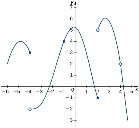
Problem 79. Use the graph shown below.
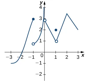
Problem 80. Use the graph to evaluate (a) \(f'(-0.5),\) (b) \(f'(0),\) (c) \(f'(1),\) (d) \(f'(2),\) and (e) \(f'(3),\) if it exists.
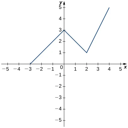
For the following functions, use \(f''(x) = \lim_{h \to 0} \dfrac{f'(x+h) - f'(x)}{h}\) to find \(f''(x).\)
Problem 81. \(f(x) = 2 - 3x\)
Problem 82. \(f(x) = 4x^2\)
Problem 83. \(f(x) = x + \dfrac{1}{x}\)
Solutions 15–30
Problem 15
Step 1 — Recognize the definition of the derivative at a point: The limit \(\displaystyle\lim_{h\to 0}\frac{f(a+h)-f(a)}{h}\) is the derivative \(f'(a)\). We need to read off \(a\) and \(f\) from the limit.
Step 2 — Identify \(a\): The expression \((1+h)^{2/3}\) has the form \((a+h)^{2/3}\), so \(a = 1\).
Step 3 — Verify \(f(a)\): The constant being subtracted is \(1\). If \(f(x) = x^{2/3}\), then \(f(1) = 1^{2/3} = 1\). ✓
Step 4 — Identify \(f\): Replacing \((1+h)\) by the variable \(x\) in the expression \((1+h)^{2/3}\) gives \(f(x) = x^{2/3}\).
Answer: \(f(x) = x^{2/3}\) and \(a = 1\).
Problem 16
Step 1 — Recognize the definition of the derivative at a point: The limit has the form \(\displaystyle\lim_{h\to 0}\frac{f(a+h)-f(a)}{h} = f'(a)\).
Step 2 — Identify \(a\): The expression \(3(2+h)^2 + 2\) has the shape \(3(a+h)^2 + 2\) with \(a = 2\).
Step 3 — Verify \(f(a)\): The constant subtracted is \(14\). If \(f(x) = 3x^2 + 2\), then \(f(2) = 3(2)^2 + 2 = 12 + 2 = 14\). ✓
Step 4 — Identify \(f\): Replacing \((2+h)\) by \(x\) in \(3(2+h)^2 + 2\) gives \(f(x) = 3x^2 + 2\).
Answer: \(f(x) = 3x^2 + 2\) and \(a = 2\).
Problem 17
Step 1 — Recognize the definition of the derivative at a point: The limit has the form \(\displaystyle\lim_{h\to 0}\frac{f(a+h)-f(a)}{h} = f'(a)\).
Step 2 — Identify \(a\): The expression \(\cos(\pi + h)\) has the form \(\cos(a + h)\) with \(a = \pi\).
Step 3 — Verify \(f(a)\): The numerator is \(\cos(\pi + h) + 1\). Rewriting \(+1\) as \(-(-1)\) and noting \(\cos(\pi) = -1\), we get \(\cos(\pi + h) - \cos(\pi)\). So the subtracted constant is \(f(\pi) = \cos(\pi) = -1\). ✓
Step 4 — Identify \(f\): Replacing \((\pi + h)\) by \(x\) in \(\cos(\pi + h)\) gives \(f(x) = \cos x\).
Answer: \(f(x) = \cos x\) and \(a = \pi\).
Problem 18
Step 1 — Recognize the definition of the derivative at a point: The limit has the form \(\displaystyle\lim_{h\to 0}\frac{f(a+h)-f(a)}{h} = f'(a)\).
Step 2 — Identify \(a\): The expression \((2+h)^4\) has the form \((a+h)^4\) with \(a = 2\).
Step 3 — Verify \(f(a)\): The constant subtracted is \(16\). If \(f(x) = x^4\), then \(f(2) = 2^4 = 16\). ✓
Step 4 — Identify \(f\): Replacing \((2+h)\) by \(x\) in \((2+h)^4\) gives \(f(x) = x^4\).
Answer: \(f(x) = x^4\) and \(a = 2\).
Problem 19
Step 1 — Recognize the definition of the derivative at a point: The limit has the form \(\displaystyle\lim_{h\to 0}\frac{f(a+h)-f(a)}{h} = f'(a)\).
Step 2 — Identify \(a\): Every occurrence of the variable in the first bracket is \((3+h)\), so \(a = 3\).
Step 3 — Verify \(f(a)\): The constant subtracted is \(15\). If \(f(x) = 2x^2 - x\), then \(f(3) = 2(3)^2 - 3 = 18 - 3 = 15\). ✓
Step 4 — Identify \(f\): Replacing \((3+h)\) by \(x\) in \(2(3+h)^2 - (3+h)\) gives \(f(x) = 2x^2 - x\).
Answer: \(f(x) = 2x^2 - x\) and \(a = 3\).
Problem 20
Step 1 — Recognize the definition of the derivative at a point: The limit has the form \(\displaystyle\lim_{h\to 0}\frac{f(a+h)-f(a)}{h} = f'(a)\).
Step 2 — Identify \(a\): The numerator \(e^h - 1\) can be written as \(e^{0+h} - 1\), so \((a+h) = (0+h)\) and \(a = 0\).
Step 3 — Verify \(f(a)\): The constant subtracted is \(1\). If \(f(x) = e^x\), then \(f(0) = e^0 = 1\). ✓
Step 4 — Identify \(f\): Replacing \((0+h) = h\) by \(x\) in \(e^h\) gives \(f(x) = e^x\).
Answer: \(f(x) = e^x\) and \(a = 0\).
Problem 21
Step 1 — Describe the graph: On \([0,1]\) the piece \(2\sqrt{x}\) is the upper half of a sideways parabola, starting at \((0,0)\) and rising with a steepening-then-flattening curve to \((1,2)\). For \(x>1\) the piece \(3x-1\) is a straight line of slope \(3\) that also passes through \((1,2)\) (open dot on the left piece's endpoint, line continuing upward to the right). The two pieces meet at \((1,2)\) so the function is continuous there, but the curve hits the corner with a noticeably steeper line than the gentle square-root slope.
Step 2 — Confirm continuity at \(x=1\): \(f(1)=2\sqrt{1}=2\) and \(\lim_{x\to 1^+}(3x-1)=2\), so \(\lim_{x\to1}f(x)=f(1)=2\).
Step 3 — Left-hand derivative at \(x=1\): Using the definition, $$f'_-(1)=\lim_{x\to 1^-}\frac{f(x)-f(1)}{x-1}=\lim_{x\to1^-}\frac{2\sqrt{x}-2}{x-1}.$$ Factor \(x-1=(\sqrt{x}-1)(\sqrt{x}+1)\): $$f'_-(1)=\lim_{x\to1^-}\frac{2(\sqrt{x}-1)}{(\sqrt{x}-1)(\sqrt{x}+1)}=\lim_{x\to1^-}\frac{2}{\sqrt{x}+1}=\frac{2}{2}=1.$$
Step 4 — Right-hand derivative at \(x=1\): $$f'_+(1)=\lim_{x\to1^+}\frac{(3x-1)-2}{x-1}=\lim_{x\to1^+}\frac{3(x-1)}{x-1}=3.$$
Step 5 — Compare: Since \(f'_-(1)=1\ne 3=f'_+(1)\), the two one-sided derivatives disagree, so the limit defining \(f'(1)\) does not exist.
Answer: \(f\) is continuous at \(x=1\) but not differentiable at \(x=1\); the left-hand derivative is \(1\) and the right-hand derivative is \(3\).
Problem 22
Step 1 — Describe the graph: For \(x<1\) the function is the constant line \(y=3\); for \(x\ge 1\) it is the line \(y=3x\), which at \(x=1\) gives \(y=3\) and rises with slope \(3\). The horizontal piece runs into the closed dot at \((1,3)\), and the second piece continues from \((1,3)\) upward as a slanted line. The two pieces meet at the same height, so the graph has a sharp corner at \((1,3)\).
Step 2 — Confirm continuity at \(x=1\): \(\lim_{x\to1^-}f(x)=3\) and \(f(1)=3(1)=3=\lim_{x\to1^+}f(x)\), so \(f\) is continuous at \(x=1\).
Step 3 — Left-hand derivative at \(x=1\): For \(x<1\), \(f(x)=3\), so $$f'_-(1)=\lim_{x\to1^-}\frac{3-3}{x-1}=\lim_{x\to1^-}0=0.$$
Step 4 — Right-hand derivative at \(x=1\): For \(x\ge 1\), \(f(x)=3x\), so $$f'_+(1)=\lim_{x\to1^+}\frac{3x-3}{x-1}=\lim_{x\to1^+}\frac{3(x-1)}{x-1}=3.$$
Step 5 — Compare: Because \(0\ne 3\), the one-sided derivatives disagree and \(f'(1)\) does not exist.
Answer: \(f\) is continuous at \(x=1\) but not differentiable at \(x=1\); \(f'_-(1)=0\) and \(f'_+(1)=3\).
Problem 23
Step 1 — Describe the graph: For \(x\le 1\) the piece \(-x^2+2\) is a downward-opening parabola with vertex at \((0,2)\); on \((-\infty,1]\) it rises on the left, peaks at \((0,2)\), then falls to \((1,1)\) (closed dot). For \(x>1\) the function is the line \(y=x\), which passes through \((1,1)\) and continues upward with slope \(1\). The pieces meet smoothly in value at \((1,1)\) but the parabola arrives with negative slope while the line departs with positive slope, producing a corner.
Step 2 — Confirm continuity at \(x=1\): \(f(1)=-(1)^2+2=1\) and \(\lim_{x\to1^+}x=1\), so \(\lim_{x\to1}f(x)=f(1)=1\).
Step 3 — Left-hand derivative at \(x=1\): $$f'_-(1)=\lim_{x\to1^-}\frac{(-x^2+2)-1}{x-1}=\lim_{x\to1^-}\frac{1-x^2}{x-1}=\lim_{x\to1^-}\frac{-(x-1)(x+1)}{x-1}=\lim_{x\to1^-}-(x+1)=-2.$$
Step 4 — Right-hand derivative at \(x=1\): $$f'_+(1)=\lim_{x\to1^+}\frac{x-1}{x-1}=1.$$
Step 5 — Compare: Since \(-2\ne 1\), the two one-sided derivatives disagree, so \(f'(1)\) does not exist.
Answer: \(f\) is continuous at \(x=1\) but not differentiable at \(x=1\); \(f'_-(1)=-2\) and \(f'_+(1)=1\).
Problem 24
Step 1 — Describe the graph: For \(x\le 1\) the piece \(2x\) is a straight line through the origin with slope \(2\), reaching \((1,2)\) (closed dot). For \(x>1\) the piece \(2/x\) is the upper branch of a hyperbola that starts (open) at \((1,2)\) and decreases toward \(0\) as \(x\to\infty\). The two pieces share the height \(2\) at \(x=1\), so the graph is continuous, but the line arrives rising while the hyperbola departs falling, leaving a sharp corner.
Step 2 — Confirm continuity at \(x=1\): \(f(1)=2(1)=2\) and \(\lim_{x\to1^+}\frac{2}{x}=2\), so \(\lim_{x\to1}f(x)=f(1)=2\).
Step 3 — Left-hand derivative at \(x=1\): $$f'_-(1)=\lim_{x\to1^-}\frac{2x-2}{x-1}=\lim_{x\to1^-}\frac{2(x-1)}{x-1}=2.$$
Step 4 — Right-hand derivative at \(x=1\): $$f'_+(1)=\lim_{x\to1^+}\frac{\frac{2}{x}-2}{x-1}=\lim_{x\to1^+}\frac{2-2x}{x(x-1)}=\lim_{x\to1^+}\frac{-2(x-1)}{x(x-1)}=\lim_{x\to1^+}\frac{-2}{x}=-2.$$
Step 5 — Compare: Since \(2\ne -2\), the two one-sided derivatives disagree and \(f'(1)\) does not exist.
Answer: \(f\) is continuous at \(x=1\) but not differentiable at \(x=1\); \(f'_-(1)=2\) and \(f'_+(1)=-2\).
Problem 25
Step 1 — Read the alt-text for the graph: From the figure, the function comes in at \((-6,2)\), rises to a maximum at \((-5.3,4)\), and stops inclusive at \((-4,3)\). It restarts at \((-4,-2)\), rises slowly through \((-2.25,0)\), passes through \((-1,4)\), peaks at \((-0.1,5.3)\), and decreases to \((2,-1)\) inclusive. The graph restarts at \((2,5)\), rises to \((2.6,6)\), then decreases to \((4.5,-3)\) with a discontinuity at \(x=4\) where the value is \(2\).
Step 2 — Find points where the limit exists but \(f\) is not continuous there: A two-sided limit can still exist at a point where the value is misplaced. Inspecting each gap, the genuine jumps at \(x=-4\) (\(3\) on the left, \(-2\) on the right) and \(x=2\) (\(-1\) on the left, \(5\) on the right) are jump discontinuities — the one-sided limits exist but disagree, so the two-sided limit does not exist. At \(x=4\) the curve continues from both sides but the plotted value is \(2\) rather than the curve's value (a removable discontinuity); here the two-sided limit exists yet \(f\) is not continuous. So the only point fitting the criterion is \(x=4\).
Step 3 — Find points where \(f\) is continuous but not differentiable: A continuous corner or vertical tangent kills differentiability. The graph shows smooth turning except at the local maximum near \((-0.1,5.3)\) and the local maximum near \((2.6,6)\); these appear smooth. The only feature on the connected middle piece where the slope of the graph changes abruptly while the curve remains unbroken is the kink around \(x=-1\) where the slow rise steepens. (No other corners on continuous segments are evident from the description.) The endpoints \(x=-4\) and \(x=2\) are discontinuities, not corners, so they are excluded.
Answer: (a) \(f\) has a removable discontinuity at \(x=4\) (the two-sided limit exists but does not equal \(f(4)\)). (b) Within the continuous middle piece the only point that looks like a corner is near \(x=-1\), where the graph is continuous but not differentiable.
Problem 26
Step 1 — Read the alt-text for the graph: The function comes in at \((-3,-1)\), rises and stops inclusive at the local maximum \((-1,3)\). It restarts at \((-1,1)\), climbs quickly and stops inclusive at the local maximum \((0,4)\). It restarts at \((0,3)\) and decreases linearly to \((1,1)\); at \(x=1\) there is a discontinuity and the plotted value \(f(1)=2\). The graph continues from \((1,1)\) and rises linearly to \((2,3.5)\), then falls linearly to \((3,2)\).
Step 2 — Points where the limit exists but \(f\) is not continuous: At \(x=-1\) the left value is \(3\) and the right value is \(1\): one-sided limits disagree, so the two-sided limit does not exist (jump). At \(x=0\) the left value is \(4\) and the right value is \(3\): another jump, so the two-sided limit does not exist. At \(x=1\) both sides of the curve approach \(1\) but the plotted value is \(2\) — the two-sided limit exists and equals \(1\), while \(f(1)=2\), so this is a removable discontinuity.
Step 3 — Points where \(f\) is continuous but not differentiable: The pieces from \((1,1)\) up to \((2,3.5)\) and down to \((3,2)\) are described as straight line segments meeting at \((2,3.5)\); the slopes (\(2.5\) on the left, \(-1.5\) on the right) disagree, producing a corner where the graph is continuous but not differentiable. No other interior corners are described.
Answer: (a) The only point where \(\lim_{x\to a}f(x)\) exists but \(f\) is not continuous is \(x=1\) (removable discontinuity). (b) \(f\) is continuous but not differentiable at \(x=2\) (corner between two line segments of differing slope).
Problem 27
Step 1 — Read the alt-text for the graph: The function starts at \((-3,0)\) and increases linearly to a local maximum at \((0,3)\); it then decreases linearly to \((2,1)\); finally it increases linearly to \((4,5)\). The graph is three connected line segments with corners at \(x=0\) and \(x=2\).
Step 2 — Compute slopes on each linear piece: - Left segment from \((-3,0)\) to \((0,3)\): slope \(=\dfrac{3-0}{0-(-3)}=1\). - Middle segment from \((0,3)\) to \((2,1)\): slope \(=\dfrac{1-3}{2-0}=-1\). - Right segment from \((2,1)\) to \((4,5)\): slope \(=\dfrac{5-1}{4-2}=2\).
Step 3 — Evaluate \(f'\) at each requested point:
(a) \(x=-0.5\): inside the left segment, so \(f'(-0.5)=1\).
(b) \(x=0\): corner where the slope jumps from \(1\) (left) to \(-1\) (right). The one-sided derivatives disagree, so \(f'(0)\) does not exist.
(c) \(x=1\): inside the middle segment, so \(f'(1)=-1\).
(d) \(x=2\): corner where the slope jumps from \(-1\) (left) to \(2\) (right). One-sided derivatives disagree, so \(f'(2)\) does not exist.
(e) \(x=3\): inside the right segment, so \(f'(3)=2\).
Answer: \(f'(-0.5)=1\); \(f'(0)\) DNE (corner); \(f'(1)=-1\); \(f'(2)\) DNE (corner); \(f'(3)=2\).
Problem 28
Step 1 — Find \(f'(x)\) from the limit definition: With \(f(x)=2-3x\), $$f'(x)=\lim_{h\to 0}\frac{f(x+h)-f(x)}{h}=\lim_{h\to 0}\frac{[2-3(x+h)]-[2-3x]}{h}=\lim_{h\to 0}\frac{-3h}{h}=-3.$$ So \(f'(x)=-3\) for all \(x\).
Step 2 — Apply the limit definition to \(f'\) to get \(f''(x)\): $$f''(x)=\lim_{h\to 0}\frac{f'(x+h)-f'(x)}{h}=\lim_{h\to 0}\frac{(-3)-(-3)}{h}=\lim_{h\to 0}\frac{0}{h}=0.$$
The numerator is identically zero because \(f'\) is constant, so the difference quotient is \(0\) for every \(h\ne 0\) and the limit is \(0\).
Answer: \(f''(x)=0\).
Problem 29
Step 1 — Find \(f'(x)\) from the limit definition: With \(f(x)=4x^2\), $$f'(x)=\lim_{h\to 0}\frac{4(x+h)^2-4x^2}{h}=\lim_{h\to 0}\frac{4(x^2+2xh+h^2)-4x^2}{h}=\lim_{h\to 0}\frac{8xh+4h^2}{h}=\lim_{h\to 0}(8x+4h)=8x.$$
Step 2 — Apply the limit definition to \(f'\) to get \(f''(x)\): With \(f'(x)=8x\), $$f''(x)=\lim_{h\to 0}\frac{f'(x+h)-f'(x)}{h}=\lim_{h\to 0}\frac{8(x+h)-8x}{h}=\lim_{h\to 0}\frac{8h}{h}=8.$$
Answer: \(f''(x)=8\).
Problem 30
Step 1 — Find \(f'(x)\) from the limit definition: With \(f(x)=x+\dfrac{1}{x}\), $$f'(x)=\lim_{h\to 0}\frac{\left[(x+h)+\frac{1}{x+h}\right]-\left[x+\frac{1}{x}\right]}{h}=\lim_{h\to 0}\left[1+\frac{1}{h}!\left(\frac{1}{x+h}-\frac{1}{x}\right)\right].$$ Combine the inner difference over a common denominator: $$\frac{1}{x+h}-\frac{1}{x}=\frac{x-(x+h)}{x(x+h)}=\frac{-h}{x(x+h)}.$$ Substituting and cancelling the \(h\): $$f'(x)=\lim_{h\to 0}\left[1+\frac{-1}{x(x+h)}\right]=1-\frac{1}{x^2}.$$
Step 2 — Apply the limit definition to \(f'\) to get \(f''(x)\): With \(f'(x)=1-\dfrac{1}{x^2}\), $$f''(x)=\lim_{h\to 0}\frac{\left[1-\frac{1}{(x+h)^2}\right]-\left[1-\frac{1}{x^2}\right]}{h}=\lim_{h\to 0}\frac{1}{h}!\left(\frac{1}{x^2}-\frac{1}{(x+h)^2}\right).$$ Common denominator inside: $$\frac{1}{x^2}-\frac{1}{(x+h)^2}=\frac{(x+h)^2-x^2}{x^2(x+h)^2}=\frac{2xh+h^2}{x^2(x+h)^2}=\frac{h(2x+h)}{x^2(x+h)^2}.$$ Divide by \(h\) and take the limit: $$f''(x)=\lim_{h\to 0}\frac{2x+h}{x^2(x+h)^2}=\frac{2x}{x^2\cdot x^2}=\frac{2}{x^3}.$$
Answer: \(f''(x)=\dfrac{2}{x^3}\).
For the following exercises, use a calculator to graph \(f(x).\) Determine the function \(f'(x),\) then use a calculator to graph \(f'(x).\)
Problem 84. [T] \(f(x) = -\dfrac{5}{x}\)
Problem 85. [T] \(f(x) = 3x^2 + 2x + 4\)
Problem 86. [T] \(f(x) = \sqrt{x} + 3x\)
Problem 87. [T] \(f(x) = \dfrac{1}{\sqrt{2x}}\)
Problem 88. [T] \(f(x) = 1 + x + \dfrac{1}{x}\)
Problem 89. [T] \(f(x) = x^3 + 1\)
- \(\dfrac{f(x+h) - f(x)}{h}\)
- \(f'(x) = \displaystyle\lim_{h \to 0} \dfrac{f(x+h) - f(x)}{h}\)
represents in terms of the given situation. Be sure to include units.
Solutions 31–36
Problem 31
Step 1 — Set up the limit definition: By definition, \(f'(x) = \lim_{h \to 0} \dfrac{f(x+h) - f(x)}{h}\). For \(f(x) = -5/x\),
$$f'(x) = \lim_{h \to 0} \frac{\dfrac{-5}{x+h} - \dfrac{-5}{x}}{h}.$$Step 2 — Combine the fractions in the numerator: Get a common denominator \(x(x+h)\):
$$\frac{-5}{x+h} + \frac{5}{x} = \frac{-5x + 5(x+h)}{x(x+h)} = \frac{5h}{x(x+h)}.$$Step 3 — Divide by \(h\) and take the limit: This gives
$$f'(x) = \lim_{h \to 0} \frac{5h}{h \cdot x(x+h)} = \lim_{h \to 0} \frac{5}{x(x+h)} = \frac{5}{x^2}.$$Step 4 — Describe the graphs: Graph of \(f(x) = -5/x\): domain \(x \ne 0\), vertical asymptote at \(x = 0\), horizontal asymptote \(y = 0\); the hyperbola sits in quadrants II and IV (positive for \(x<0\), negative for \(x>0\)). Graph of \(f'(x) = 5/x^2\): domain \(x \ne 0\), vertical asymptote at \(x = 0\), horizontal asymptote \(y = 0\); always positive, so \(f\) is increasing on each piece of its domain.
Note on the graphing calculator: Entering \(Y_1 = -5/X\) and \(Y_2 = 5/X^2\) on a standard window shows the hyperbola for \(Y_1\) with branches in quadrants II and IV, and \(Y_2\) as a strictly positive curve with both branches rising toward the \(y\)-axis.
Answer: \(f'(x) = \dfrac{5}{x^2}\).
Problem 32
Step 1 — Form the difference quotient: With \(f(x) = 3x^2 + 2x + 4\),
$$f(x+h) = 3(x+h)^2 + 2(x+h) + 4 = 3x^2 + 6xh + 3h^2 + 2x + 2h + 4.$$Step 2 — Subtract \(f(x)\) and simplify:
$$f(x+h) - f(x) = 6xh + 3h^2 + 2h.$$Step 3 — Divide by \(h\) and take the limit:
$$f'(x) = \lim_{h \to 0} \frac{6xh + 3h^2 + 2h}{h} = \lim_{h \to 0} (6x + 3h + 2) = 6x + 2.$$Step 4 — Describe the graphs: Graph of \(f\): an upward-opening parabola with \(y\)-intercept \(4\); vertex where \(6x + 2 = 0\), i.e. \(x = -1/3\), giving vertex \((-1/3, 11/3)\); decreasing on \((-\infty, -1/3)\), increasing on \((-1/3, \infty)\). Graph of \(f'(x) = 6x + 2\): a straight line with slope \(6\) and \(y\)-intercept \(2\); crosses zero at \(x = -1/3\), matching the parabola's vertex.
Note on the graphing calculator: Plotting \(Y_1 = 3X^2 + 2X + 4\) and \(Y_2 = 6X + 2\) together shows the parabola with its minimum directly above the \(x\)-intercept of the line.
Answer: \(f'(x) = 6x + 2\).
Problem 33
Step 1 — Set up the limit definition: With \(f(x) = \sqrt{x} + 3x\),
$$f'(x) = \lim_{h \to 0} \frac{\sqrt{x+h} + 3(x+h) - \sqrt{x} - 3x}{h} = \lim_{h \to 0} \left( \frac{\sqrt{x+h} - \sqrt{x}}{h} + 3 \right).$$Step 2 — Rationalize the square-root piece: Multiply by the conjugate:
$$\frac{\sqrt{x+h} - \sqrt{x}}{h} \cdot \frac{\sqrt{x+h} + \sqrt{x}}{\sqrt{x+h} + \sqrt{x}} = \frac{(x+h) - x}{h(\sqrt{x+h} + \sqrt{x})} = \frac{1}{\sqrt{x+h} + \sqrt{x}}.$$Step 3 — Take the limit: As \(h \to 0\), \(\sqrt{x+h} \to \sqrt{x}\), so
$$f'(x) = \frac{1}{2\sqrt{x}} + 3.$$Step 4 — Describe the graphs: Graph of \(f(x) = \sqrt{x} + 3x\): domain \(x \ge 0\), passes through the origin, strictly increasing, concave down because the \(\sqrt{x}\) curvature dominates near zero while the line \(3x\) takes over for large \(x\). Graph of \(f'(x) = \tfrac{1}{2\sqrt{x}} + 3\): domain \(x > 0\), vertical asymptote at \(x = 0\) (the slope is infinite there), always greater than \(3\), and decreases monotonically toward the horizontal asymptote \(y = 3\) as \(x \to \infty\).
Note on the graphing calculator: \(Y_1 = \sqrt{X} + 3X\) shows a rising curve starting at the origin; \(Y_2 = 1/(2\sqrt{X}) + 3\) spikes near \(x = 0\) and flattens toward the line \(y = 3\).
Answer: \(f'(x) = \dfrac{1}{2\sqrt{x}} + 3\), with domain \(x > 0\).
Problem 34
Step 1 — Set up the limit: With \(f(x) = \dfrac{1}{\sqrt{2x}}\),
$$f'(x) = \lim_{h \to 0} \frac{\dfrac{1}{\sqrt{2(x+h)}} - \dfrac{1}{\sqrt{2x}}}{h}.$$Step 2 — Combine the fractions in the numerator: Common denominator \(\sqrt{2x}\sqrt{2(x+h)}\):
$$\frac{1}{\sqrt{2(x+h)}} - \frac{1}{\sqrt{2x}} = \frac{\sqrt{2x} - \sqrt{2(x+h)}}{\sqrt{2x}\,\sqrt{2(x+h)}}.$$Step 3 — Rationalize using the conjugate: Multiply by \(\dfrac{\sqrt{2x} + \sqrt{2(x+h)}}{\sqrt{2x} + \sqrt{2(x+h)}}\):
$$\frac{2x - 2(x+h)}{\sqrt{2x}\,\sqrt{2(x+h)}\,\bigl(\sqrt{2x} + \sqrt{2(x+h)}\bigr)} = \frac{-2h}{\sqrt{2x}\,\sqrt{2(x+h)}\,\bigl(\sqrt{2x} + \sqrt{2(x+h)}\bigr)}.$$Step 4 — Divide by \(h\) and take the limit:
$$f'(x) = \lim_{h \to 0} \frac{-2}{\sqrt{2x}\,\sqrt{2(x+h)}\,\bigl(\sqrt{2x} + \sqrt{2(x+h)}\bigr)} = \frac{-2}{\sqrt{2x}\cdot\sqrt{2x}\cdot 2\sqrt{2x}} = \frac{-2}{2x \cdot 2\sqrt{2x}} = \frac{-1}{2x\sqrt{2x}}.$$Step 5 — Describe the graphs: Graph of \(f(x) = 1/\sqrt{2x}\): domain \(x > 0\), vertical asymptote at \(x = 0\), horizontal asymptote \(y = 0\); strictly decreasing and positive. Graph of \(f'(x) = -1/(2x\sqrt{2x})\): same domain, vertical asymptote at \(x = 0\) heading to \(-\infty\), horizontal asymptote \(y = 0\) from below; always negative, matching \(f\)'s decreasing behavior.
Note on the graphing calculator: Entering \(Y_1 = 1/\sqrt{2X}\) and \(Y_2 = -1/(2X\sqrt{2X})\) shows a positive decreasing curve and a negative curve that mirrors it across the \(x\)-axis, both with the same \(y\)-axis asymptote.
Answer: \(f'(x) = -\dfrac{1}{2x\sqrt{2x}} = -\dfrac{\sqrt{2}}{4\, x^{3/2}}\), with domain \(x > 0\).
Problem 35
Step 1 — Form the difference quotient: With \(f(x) = 1 + x + 1/x\),
$$f(x+h) - f(x) = (x+h) - x + \frac{1}{x+h} - \frac{1}{x} = h + \frac{x - (x+h)}{x(x+h)} = h - \frac{h}{x(x+h)}.$$Step 2 — Divide by \(h\):
$$\frac{f(x+h) - f(x)}{h} = 1 - \frac{1}{x(x+h)}.$$Step 3 — Take the limit: As \(h \to 0\), \(x(x+h) \to x^2\), so
$$f'(x) = 1 - \frac{1}{x^2}.$$Step 4 — Describe the graphs: Graph of \(f(x) = 1 + x + 1/x\): domain \(x \ne 0\), vertical asymptote at \(x = 0\), oblique asymptote \(y = 1 + x\); local max at \(x = -1\) (value \(-1\)), local min at \(x = 1\) (value \(3\)). Graph of \(f'(x) = 1 - 1/x^2\): domain \(x \ne 0\), horizontal asymptote \(y = 1\), vertical asymptote at \(x = 0\) heading to \(-\infty\); zeros at \(x = \pm 1\), positive for \(|x| > 1\) and negative for \(0 < |x| < 1\), confirming the monotonicity of \(f\).
Note on the graphing calculator: \(Y_1 = 1 + X + 1/X\) shows two branches with a local max in the third quadrant and a local min in the first; \(Y_2 = 1 - 1/X^2\) crosses the \(x\)-axis at \(\pm 1\) and approaches the line \(y = 1\).
Answer: \(f'(x) = 1 - \dfrac{1}{x^2}\), with domain \(x \ne 0\).
Problem 36
Step 1 — Expand \(f(x+h)\): With \(f(x) = x^3 + 1\),
$$f(x+h) = (x+h)^3 + 1 = x^3 + 3x^2 h + 3x h^2 + h^3 + 1.$$Step 2 — Subtract \(f(x)\) and simplify:
$$f(x+h) - f(x) = 3x^2 h + 3x h^2 + h^3.$$Step 3 — Divide by \(h\) and take the limit:
$$f'(x) = \lim_{h \to 0} \bigl(3x^2 + 3xh + h^2\bigr) = 3x^2.$$Step 4 — Describe the graphs: Graph of \(f(x) = x^3 + 1\): domain all real numbers, \(y\)-intercept \(1\), \(x\)-intercept \(-1\); strictly increasing with an inflection point at \((0, 1)\). Graph of \(f'(x) = 3x^2\): domain all real numbers, vertex at the origin, opens upward; always non-negative and zero only at \(x = 0\), confirming that \(f\) is increasing everywhere but has a horizontal tangent at the origin.
Note on the graphing calculator: \(Y_1 = X^3 + 1\) shows the standard cubic shifted up by 1; \(Y_2 = 3X^2\) shows a parabola that touches the \(x\)-axis exactly where the cubic flattens out.
Answer: \(f'(x) = 3x^2\).
For the following exercises, describe what each of the two expressions
Problem 90. \(P(x)\) denotes the population of a city at time \(x\) in years.
Problem 91. \(C(x)\) denotes the total amount of money (in thousands of dollars) spent on concessions by \(x\) customers at an amusement park.
Problem 92. \(R(x)\) denotes the total cost (in thousands of dollars) of manufacturing \(x\) clock radios.
Problem 93. \(g(x)\) denotes the grade (in percentage points) received on a test, given \(x\) hours of studying.
Problem 94. \(B(x)\) denotes the cost (in dollars) of a sociology textbook at university bookstores in the United States in \(x\) years since \(1990.\)
Problem 95. \(p(x)\) denotes atmospheric pressure in Torrs at an altitude of \(x\) feet.
Problem 96. Sketch the graph of a function \(y = f(x)\) with all of the following properties:
a) \(f'(x) > 0\) for \(-2 \le x < 1\)
b) \(f'(2) = 0\)
c) \(f'(x) > 0\) for \(x > 2\)
d) \(f(2) = 2\) and \(f(0) = 1\)
e) \(\displaystyle\lim_{x \to -\infty} f(x) = 0\) and \(\displaystyle\lim_{x \to \infty} f(x) = \infty\)
f) \(f'(1)\) does not exist.
Problem 97. Suppose temperature \(T\) in degrees Fahrenheit at a height \(x\) in feet above the ground is given by \(y = T(x).\)
a) Give a physical interpretation, with units, of \(T'(x).\)
b) If we know that \(T'(1000) = -0.1,\) explain the physical meaning.
Problem 98. Suppose the total profit of a company is \(y = P(x)\) thousand dollars when \(x\) units of an item are sold.
a) What does \(\dfrac{P(b) - P(a)}{b - a}\) for \(0 < a < b\) measure, and what are the units?
b) What does \(P'(x)\) measure, and what are the units?
c) Suppose that \(P'(30) = 5.\) What is the approximate change in profit if the number of items sold increases from \(30\) to \(31?\)
Problem 99. The graph in the following figure models the number of people \(N(t)\) who have come down with the flu \(t\) weeks after its initial outbreak in a town with a population of \(50{,}000\) citizens.
a) Describe what \(N'(t)\) represents and how it behaves as \(t\) increases.
b) What does the derivative tell us about how this town is affected by the flu outbreak?
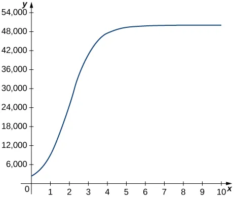
Solutions 37–46
Problem 37
Step 1 — Identify expression (1): \(\dfrac{P(x+h) - P(x)}{h}\) is the change in population \(P(x+h) - P(x)\) divided by the change in time \(h\). It measures the average rate of population growth between year \(x\) and year \(x+h\).
Step 2 — Identify expression (2): \(P'(x) = \lim_{h \to 0} \dfrac{P(x+h) - P(x)}{h}\) is the limit of those average rates as the time interval shrinks to zero. It measures the instantaneous rate of population growth at the instant \(x\) years.
Step 3 — State the units: Population is measured in people and \(x\) is measured in years, so both expressions have units of people per year.
Answer: Expression (1) is the average growth rate of the population (people/year) over the interval from \(x\) to \(x+h\) years; expression (2) is the instantaneous population growth rate (people/year) at time \(x\) years.
Problem 38
Step 1 — Identify expression (1): \(\dfrac{C(x+h) - C(x)}{h}\) is the change in concession spending (in thousands of dollars) divided by the change in number of customers \(h\). It measures the average change in concession spending per additional customer between \(x\) and \(x+h\) customers.
Step 2 — Identify expression (2): \(C'(x) = \lim_{h \to 0} \dfrac{C(x+h) - C(x)}{h}\) is the instantaneous version — the marginal concession spending when the customer count is \(x\): the extra spending generated by one more customer at that level.
Step 3 — State the units: \(C\) is measured in thousands of dollars and \(x\) in customers, so both expressions have units of thousands of dollars per customer.
Answer: Expression (1) is the average spending per additional customer (thousands of dollars per customer) over \(x\) to \(x+h\) customers; expression (2) is the marginal (instantaneous) concession-spending rate at \(x\) customers, in thousands of dollars per customer.
Problem 39
Step 1 — Identify expression (1): \(\dfrac{R(x+h) - R(x)}{h}\) is the change in manufacturing cost (in thousands of dollars) divided by the change in production level \(h\). It measures the average cost per additional clock radio when output rises from \(x\) to \(x+h\) radios.
Step 2 — Identify expression (2): \(R'(x) = \lim_{h \to 0} \dfrac{R(x+h) - R(x)}{h}\) is the marginal cost — the instantaneous cost of producing one more radio when the current production level is \(x\) radios.
Step 3 — State the units: \(R\) is measured in thousands of dollars and \(x\) in radios, so both expressions have units of thousands of dollars per radio.
Answer: Expression (1) is the average cost per extra radio (thousands of dollars per radio) over the interval \(x\) to \(x+h\); expression (2) is the marginal cost at production level \(x\), in thousands of dollars per radio.
Problem 40
Step 1 — Identify expression (1): \(\dfrac{g(x+h) - g(x)}{h}\) is the change in grade (in percentage points) divided by the change in study time \(h\) (in hours). It measures the average improvement in grade per hour of study between \(x\) and \(x+h\) hours.
Step 2 — Identify expression (2): \(g'(x) = \lim_{h \to 0} \dfrac{g(x+h) - g(x)}{h}\) is the instantaneous rate of grade improvement at \(x\) hours of study — how fast the grade is rising per additional hour right at that moment.
Step 3 — State the units: \(g\) is in percentage points (percent) and \(x\) is in hours, so both expressions have units of percentage points per hour (or "percent per hour").
Answer: Expression (1) is the average gain in grade (percentage points per hour) over the interval from \(x\) to \(x+h\) hours of study; expression (2) is the instantaneous rate of grade improvement at \(x\) hours of study, in percentage points per hour.
Problem 41
Step 1 — Identify expression (1): \(\dfrac{B(x+h) - B(x)}{h}\) is the change in textbook price (in dollars) divided by the change in time \(h\) (in years). It measures the average rate of textbook-price increase from year \(x\) to year \(x+h\) (where \(x\) is years since 1990).
Step 2 — Identify expression (2): \(B'(x) = \lim_{h \to 0} \dfrac{B(x+h) - B(x)}{h}\) is the instantaneous rate of change of the textbook price at the year corresponding to \(x\) years past 1990.
Step 3 — State the units: \(B\) is in dollars and \(x\) is in years, so both expressions have units of dollars per year.
Answer: Expression (1) is the average rate of textbook price change (dollars per year) over the interval from year \(x\) to year \(x+h\) past 1990; expression (2) is the instantaneous rate of textbook price change (dollars per year) at year \(x\).
Problem 42
Step 1 — Identify expression (1): \(\dfrac{p(x+h) - p(x)}{h}\) is the change in atmospheric pressure (in Torrs) divided by the change in altitude \(h\) (in feet). It measures the average rate of change of atmospheric pressure over the altitude interval from \(x\) to \(x+h\) feet.
Step 2 — Identify expression (2): \(p'(x) = \lim_{h \to 0} \dfrac{p(x+h) - p(x)}{h}\) is the instantaneous rate of change of atmospheric pressure with respect to altitude at altitude \(x\) feet.
Step 3 — State the units and sign: \(p\) is in Torrs and \(x\) is in feet, so both expressions have units of Torrs per foot. Because atmospheric pressure decreases as altitude increases, both quantities are negative.
Answer: Expression (1) is the average pressure change (Torrs per foot, negative) over the altitude range from \(x\) to \(x+h\) feet; expression (2) is the instantaneous rate of pressure change at altitude \(x\) feet, in Torrs per foot (also negative).
Problem 43
Step 1 — List the structural features the graph must show: We need a curve that satisfies six simultaneous conditions: positive slope on \([-2, 1)\), a non-differentiable point at \(x=1\), a horizontal tangent at \(x=2\), positive slope for \(x>2\), the two anchor values \(f(0)=1\) and \(f(2)=2\), and the horizontal asymptote \(y=0\) as \(x\to -\infty\) together with \(f(x)\to\infty\) as \(x\to\infty\).
Step 2 — Build the left tail (\(x \to -\infty\) up to \(x=-2\)): Because \(\lim_{x\to-\infty} f(x) = 0\), the graph must hug the \(x\)-axis far to the left, approaching \(y=0\) from above (or below). Bring the curve up smoothly toward the point \((-2, f(-2))\); the slope is non-negative here so the curve is already turning upward as it leaves the asymptote.
Step 3 — Increase on \([-2, 1)\): From \(x=-2\) to just before \(x=1\), draw a strictly increasing arc (slope positive everywhere on this interval). Pass through \((0,1)\) as required by \(f(0)=1\). Let the arc climb to a peak value at \(x=1\) — say the curve reaches the point \((1, 3)\) from the left.
Step 4 — Insert the non-differentiable point at \(x=1\): At \(x=1\), \(f'(1)\) must fail to exist. The cleanest way is a corner: the left-hand slope is positive (we just finished an increasing arc), and the right-hand slope is negative (we will now go down toward \((2,2)\)). The left and right tangent slopes disagree, so \(f'(1)\) does not exist. Place the corner at \((1, 3)\).
Step 5 — Decrease from the corner to \((2, 2)\) with a horizontal tangent at \(x=2\): On the interval \((1, 2)\), draw a smooth decreasing arc from \((1, 3)\) down to \((2, 2)\). The arc must flatten out as it reaches \(x=2\) so that \(f'(2)=0\) (horizontal tangent at the point \((2, 2)\)). Think of this piece as the right half of a downward-opening parabola whose vertex sits at \((2, 2)\).
Step 6 — Increase on \((2, \infty)\) with \(f(x)\to\infty\): For \(x>2\), the slope is positive again, so the curve leaves \((2, 2)\) flatly (because of the horizontal tangent) and then climbs without bound as \(x\to\infty\). The curve has another horizontal-tangent moment at \(x=2\) (a local minimum on the piece \(x\geq 1\)) before rising to \(+\infty\).
Step 7 — Sanity check every requirement: (a) \(f'(x)>0\) on \([-2,1)\) — increasing arc, check. (b) \(f'(2)=0\) — built in as the vertex tangent at \((2,2)\), check. (c) \(f'(x)>0\) for \(x>2\) — climbing arc, check. (d) \(f(0)=1\) and \(f(2)=2\) — anchored, check. (e) \(\lim_{x\to-\infty}f(x)=0\) and \(\lim_{x\to\infty}f(x)=\infty\) — left asymptote at \(y=0\), right end unbounded, check. (f) \(f'(1)\) DNE — corner at \((1,3)\), check.
Answer: A valid sketch: from the left, the graph rises out of the horizontal asymptote \(y=0\), passes through \((0,1)\), climbs to a sharp corner at \((1, 3)\) (so \(f'(1)\) does not exist), descends to a smooth horizontal-tangent minimum at \((2, 2)\), then increases without bound to the right. Label the asymptote \(y=0\) on the left, the corner at \(x=1\), and the horizontal tangent at \(x=2\).
Problem 44
Step 1 — Identify the variables and what the derivative measures: \(T\) is temperature in degrees Fahrenheit and \(x\) is altitude in feet. The derivative \(T'(x)\) is the instantaneous rate of change of temperature with respect to altitude — that is, how fast the temperature is changing per additional foot of height.
Step 2 — Read off the units of \(T'(x)\): The units of any derivative \(dy/dx\) are (units of \(y\)) per (unit of \(x\)). Here that is degrees Fahrenheit per foot (\(^\circ\)F/ft).
Step 3 — Interpret \(T'(1000) = -0.1\): At an altitude of \(1000\) feet, the temperature is changing at a rate of \(-0.1\) \(^\circ\)F per foot. The negative sign says the temperature is decreasing as altitude increases. Concretely: climbing from \(1000\) ft to \(1001\) ft drops the temperature by roughly \(0.1\) \(^\circ\)F.
Answer: (a) \(T'(x)\) is the rate of change of air temperature with respect to altitude, measured in \(^\circ\)F per foot. (b) At \(1000\) ft up, the temperature is dropping by about \(0.1\) \(^\circ\)F for every additional foot of elevation gained.
Problem 45
Step 1 — Set up the average rate of change: The difference quotient \(\dfrac{P(b)-P(a)}{b-a}\) measures the average rate of change of profit between selling \(a\) units and selling \(b\) units. Because \(P\) is measured in thousands of dollars and \(x\) in units sold, the units of this ratio are (thousand dollars)/(unit) — i.e., thousand dollars per unit sold on average over the interval from \(a\) to \(b\).
Step 2 — Take the limit to interpret \(P'(x)\): \(P'(x)\) is the instantaneous rate of change of profit with respect to the number of units sold. In business this quantity is called marginal profit: it estimates the additional profit generated by selling one more unit when current sales are \(x\). Units: thousand dollars per unit.
Step 3 — Interpret \(P'(30)=5\): At a sales level of \(30\) units, the marginal profit is \(5\) thousand dollars per unit. The linear-approximation reading: selling the 31st unit (one more than 30) is expected to add roughly \(5\) thousand dollars to profit, i.e. about $5{,}000.
Answer: (a) \(\dfrac{P(b)-P(a)}{b-a}\) is the average rate of change of profit over the sales interval \([a,b]\), in thousand dollars per unit. (b) \(P'(x)\) is the marginal profit — the instantaneous rate of profit per additional unit at the sales level \(x\), in thousand dollars per unit. (c) Selling the 31st unit (one beyond \(x=30\)) is expected to add about $5{,}000 to profit.
Problem 46
Step 1 — Interpret \(N'(t)\): \(N(t)\) counts people infected by the flu \(t\) weeks after the outbreak begins. Its derivative \(N'(t)\) is the rate of change of the infected count with respect to time — i.e., how many new infections are accumulating per week. Units: people per week.
Step 2 — Describe the qualitative behavior of \(N'(t)\): Early in the outbreak \(N(t)\) is small but climbs quickly because nearly the whole town is susceptible — so \(N'(t)\) starts out large and growing. As more of the town becomes infected, the pool of susceptible people shrinks, transmissions slow, and \(N'(t)\) decreases. Eventually, as \(N(t)\) approaches the town's population of \(50{,}000\), \(N'(t)\to 0\) — no one left to infect.
Step 3 — Locate the peak rate: \(N'(t)\) reaches its maximum at the inflection point of \(N(t)\) — the moment the epidemic curve switches from concave up (accelerating spread) to concave down (decelerating spread). Before that point, the outbreak is intensifying; after it, the outbreak is winding down even though \(N\) is still increasing.
Step 4 — Tell the story the derivative tells: \(N'(t)\) describes the speed and momentum of the outbreak. It tells public-health officials when transmission is accelerating, when it has peaked (the worst week), and when the outbreak is in retreat. The function \(N(t)\) itself only says how many are sick; the derivative says how fast that number is changing — and that is the quantity that determines hospital surge planning.
Answer: (a) \(N'(t)\) is the number of new infections per week at time \(t\); it is large early in the outbreak, peaks at the inflection point of \(N(t)\), then decreases toward \(0\) as \(N(t)\to 50{,}000\). (b) The derivative captures how fast the flu is spreading at each moment — when transmission is accelerating, when it peaks, and when it is in decline.
For the following exercises, use the following table, which shows the height \(h\) of the Saturn V rocket for the Apollo 11 mission \(t\) seconds after launch.
Problem 100. What is the physical meaning of \(h'(t)?\) What are the units?
Problem 101. [T] Construct a table of values for \(h'(t)\) and graph both \(h(t)\) and \(h'(t)\) on the same graph. (Hint: for interior points, estimate both the left limit and right limit and average them. An interior point of an interval \(I\) is an element of \(I\) which is not an endpoint of \(I.\))
Problem 102. [T] The best linear fit to the data is given by \(H(t) = 7.229t - 4.905,\) where \(H\) is the height of the rocket (in meters) and \(t\) is the time elapsed since takeoff. From this equation, determine \(H'(t).\) Graph \(H(t)\) with the given data and, on a separate coordinate plane, graph \(H'(t).\)
Problem 103. [T] The best quadratic fit to the data is given by \(G(t) = 1.429 t^2 + 0.0857 t - 0.1429,\) where \(G\) is the height of the rocket (in meters) and \(t\) is the time elapsed since takeoff. From this equation, determine \(G'(t).\) Graph \(G(t)\) with the given data and, on a separate coordinate plane, graph \(G'(t).\)
Problem 104. [T] The best cubic fit to the data is given by \(F(t) = 0.2037 t^3 + 2.956 t^2 - 2.705 t + 0.4683,\) where \(F\) is the height of the rocket (in meters) and \(t\) is the time elapsed since takeoff. From this equation, determine \(F'(t).\) Graph \(F(t)\) with the given data and, on a separate coordinate plane, graph \(F'(t).\) Does the linear, quadratic, or cubic function fit the data best?
Problem 105. Using the best linear, quadratic, and cubic fits to the data, determine what \(H''(t),\) \(G''(t),\) and \(F''(t)\) are. What are the physical meanings of \(H''(t),\) \(G''(t),\) and \(F''(t),\) and what are their units?
Solutions 47–52
Problem 47
Step 1 — Identify the variables: \(h(t)\) is the rocket's altitude at time \(t\) seconds after launch, measured in meters. The derivative \(h'(t)\) is the rate of change of altitude with respect to time.
Step 2 — Name the physical quantity: The rate of change of position with respect to time is velocity. So \(h'(t)\) is the rocket's instantaneous vertical velocity at time \(t\). Because the rocket is climbing, \(h'(t)>0\) during powered ascent.
Step 3 — Read off the units: Units of \(h'(t)\) are (units of \(h\))/(units of \(t\)) = meters per second (m/s).
Answer: \(h'(t)\) is the rocket's instantaneous vertical velocity at time \(t\), measured in meters per second (m/s).
Problem 48
Step 1 — Note on the data: The Saturn V altitude table referenced in the problem is missing from the extracted source. The procedure below applies to any equally-spaced \((t, h(t))\) table; once the rows are filled in, the same arithmetic produces the numeric \(h'(t)\) column.
Step 2 — Approximate \(h'(t)\) at interior points by central difference: For each interior time \(t_i\) where \(t_{i-1}\) and \(t_{i+1}\) are listed in the table, use $$h'(t_i) \;\approx\; \frac{h(t_{i+1}) - h(t_{i-1})}{t_{i+1} - t_{i-1}}.$$ The central difference is the average slope over the two adjacent intervals; it is more accurate than a one-sided difference because the errors from the left interval and the right interval partially cancel.
Step 3 — Handle the endpoints with one-sided differences: At the first time \(t_0\) there is no left neighbor, so use the forward difference $$h'(t_0) \;\approx\; \frac{h(t_1) - h(t_0)}{t_1 - t_0}.$$ At the last time \(t_n\) there is no right neighbor, so use the backward difference $$h'(t_n) \;\approx\; \frac{h(t_n) - h(t_{n-1})}{t_n - t_{n-1}}.$$
Step 4 — Assemble the derivative table: Build a two-column table whose left column is the same \(t\)-values as in the original altitude table and whose right column is the approximate \(h'(t)\) values from Steps 2–3. The resulting column is the numerical-derivative estimate of the rocket's velocity at each tabulated time.
Step 5 — Note on the graphing calculator:
Enter the original \((t, h)\) data into list pairs L1/L2, then create L3 of length matching L1 by computing forward/central/backward differences as above (e.g. L3(I) = (L2(I+1) - L2(I-1))/(L1(I+1) - L1(I-1)) for interior indices). Use STAT PLOT to scatter-plot (L1, L2) for \(h(t)\) and (L1, L3) for \(h'(t)\) on the same axes. The \(h(t)\) plot rises steeply (climbing altitude); the \(h'(t)\) plot rises too, but slower — it shows the velocity increasing with time, consistent with a rocket under thrust.
Answer: Use the central-difference formula \(h'(t_i)\approx[h(t_{i+1})-h(t_{i-1})]/[t_{i+1}-t_{i-1}]\) at interior points and forward/backward differences at the endpoints; tabulate the result alongside \(t\), then plot both \(h(t)\) and \(h'(t)\) versus \(t\). \(h(t)\) is monotone increasing and concave up; \(h'(t)\) is positive and increasing — the rocket is gaining altitude and accelerating.
Problem 49
Step 1 — Differentiate the linear model: Given the regression line $$H(t) = 7.229\,t - 4.905,$$ apply the power rule term-by-term: $$H'(t) = 7.229.$$ The derivative is a constant — the slope of the regression line itself.
Step 2 — Physical interpretation: A constant derivative \(H'(t) = 7.229\) m/s says the linear fit models the rocket as moving with a constant velocity of about \(7.229\) meters per second throughout the entire interval. Equivalently, the rocket gains \(7.229\) meters of altitude every second, every second.
Step 3 — Reality check: This is physically unrealistic. A real rocket starts at rest and accelerates as its engines push it upward; its velocity grows monotonically with time. The linear model averages out that acceleration into a single mean velocity. It will under-predict velocity early in flight and over-predict it late in flight, but it captures the overall altitude gain on average.
Step 4 — Note on the graphing calculator: On the calculator, graphing \(H'(t)\) produces a horizontal line at \(y = 7.229\) — \(H'\) does not vary with \(t\). Overlaying the actual \((t, h(t))\) scatter on \(H(t)\) shows the points hugging a straight line; overlaying the numerically estimated \(h'(t)\) values on \(H'(t)=7.229\) shows the numerical velocities scattered around (and crossing) that horizontal line.
Answer: \(H'(t) = 7.229\) m/s. The linear regression treats the rocket's velocity as a constant \(7.229\) m/s throughout the climb — a coarse summary that ignores acceleration. On a graph, \(H'(t)\) is a horizontal line at \(y = 7.229\).
Problem 50
Step 1 — Differentiate the quadratic model: Given $$G(t) = 1.429\,t^{2} + 0.0857\,t - 0.1429,$$ apply the power rule term by term: $$G'(t) = 2(1.429)\,t + 0.0857 - 0 = 2.858\,t + 0.0857.$$
Step 2 — Physical interpretation of \(G'(t)\): \(G'(t)\) is a linear function of \(t\): the velocity grows in proportion to time. In physics this is the hallmark of uniform (constant) acceleration — the rocket speeds up at a steady rate. At \(t=0\) the model predicts a velocity of \(0.0857\) m/s (essentially at rest), and the velocity increases by \(2.858\) m/s for every additional second of flight.
Step 3 — Compare with the linear fit: Where the linear model \(H\) said velocity was constant, the quadratic model \(G\) says velocity grows linearly. This is more realistic: a rocket under steady thrust against (approximately) constant gravity does accelerate, and the quadratic model captures that with a single constant acceleration of \(2.858\) m/s\(^2\).
Step 4 — Note on the graphing calculator: Graphing \(G'(t) = 2.858t + 0.0857\) produces a straight line through the \(y\)-intercept \((0, 0.0857)\) with slope \(2.858\). Overlaying the numerically estimated \(h'(t)\) data from problem 3.2.48 on top of this line shows the data points clustered around the line — the velocity rises linearly with \(t\), as the quadratic fit predicts.
Answer: \(G'(t) = 2.858\,t + 0.0857\) m/s. Physically, the quadratic fit models the rocket as uniformly accelerating: velocity grows linearly with time, with constant acceleration \(2.858\) m/s\(^2\). The graph of \(G'(t)\) is the line through \((0, 0.0857)\) with slope \(2.858\).
Problem 51
Step 1 — Differentiate the cubic model: Given $$F(t) = 0.2037\,t^{3} + 2.956\,t^{2} - 2.705\,t + 0.4683,$$ apply the power rule to each term: $$F'(t) = 3(0.2037)\,t^{2} + 2(2.956)\,t - 2.705 = 0.6111\,t^{2} + 5.912\,t - 2.705.$$
Step 2 — Physical interpretation of \(F'(t)\): \(F'(t)\) is a quadratic function of \(t\), so the velocity itself grows quadratically. That allows the acceleration (the next derivative) to vary with \(t\) — which is precisely what a real rocket does. As the rocket burns fuel, its mass drops, so the same thrust produces ever-increasing acceleration; the cubic fit is flexible enough to capture this changing acceleration where the linear and quadratic fits cannot.
Step 3 — Shape of the \(F'(t)\) graph: Because the leading coefficient \(0.6111>0\), the graph of \(F'(t)\) is an upward-opening parabola. Its vertex lies at $$t_{\text{vertex}} = -\frac{5.912}{2(0.6111)} \approx -4.84,$$ which is to the left of the data window (\(t\ge 0\)), so on the data interval \(F'(t)\) is strictly increasing. The velocity grows fastest late in the climb — consistent with a rocket shedding fuel mass during ascent.
Step 4 — Why the cubic fit is the best of the three: The linear model has zero acceleration; the quadratic has constant acceleration; only the cubic permits acceleration to change over time. Real Saturn V flight data show velocity increasing super-linearly during the powered-ascent phase, so the cubic captures the trend the other two models smooth away.
Step 5 — Note on the graphing calculator: Plot \(Y_1 = 0.6111X^{2} + 5.912X - 2.705\) on \([0, T]\) for whatever time window the table covers. The screen shows an upward-curving arc rising from \(F'(0)=-2.705\) (a small negative or near-zero value at launch, an artifact of the cubic fit on noisy early data) to a much larger positive value at the end. Overlaying the numerical \(h'(t)\) estimates from problem 3.2.48 shows the data points hugging this curve more tightly than they hug the line from problem 3.2.50.
Answer: \(F'(t) = 0.6111\,t^{2} + 5.912\,t - 2.705\) m/s. The cubic regression lets velocity grow quadratically with time, allowing the acceleration to change — the most physically realistic of the three fits, matching a rocket that accelerates harder as it burns off fuel. Graph: an upward-opening parabola, increasing on the data window.
Problem 52
Step 1 — Differentiate each model twice: Start from the three fits and take two derivatives in succession.
Linear: $$H(t) = 7.229\,t - 4.905 \;\Longrightarrow\; H'(t) = 7.229 \;\Longrightarrow\; H''(t) = 0.$$
Quadratic: $$G(t) = 1.429\,t^{2} + 0.0857\,t - 0.1429 \;\Longrightarrow\; G'(t) = 2.858\,t + 0.0857 \;\Longrightarrow\; G''(t) = 2.858.$$
Cubic: $$F(t) = 0.2037\,t^{3} + 2.956\,t^{2} - 2.705\,t + 0.4683 \;\Longrightarrow\; F'(t) = 0.6111\,t^{2} + 5.912\,t - 2.705 \;\Longrightarrow\; F''(t) = 1.2222\,t + 5.912.$$
Step 2 — Identify each second derivative as an acceleration: The first derivative of altitude is velocity, so the second derivative of altitude is acceleration — rate of change of velocity with respect to time. Units: meters per second\(^{2}\) (m/s\(^{2}\)) for all three.
Step 3 — Interpret \(H''(t) = 0\): The linear altitude model has zero acceleration. It models the rocket as moving at a constant velocity. Physically this is unrealistic — a real rocket on the launchpad is not coasting at \(7.229\) m/s; it starts at rest and accelerates.
Step 4 — Interpret \(G''(t) = 2.858\): The quadratic altitude model has constant acceleration \(2.858\) m/s\(^{2}\). This matches the physics of an object under a constant net force — analogous to a body in uniform gravitational free-fall, but here the constant is the average effective acceleration of the rocket over the data window. More realistic than \(H''\), but still misses the fact that real rockets accelerate harder as they get lighter.
Step 5 — Interpret \(F''(t) = 1.2222\,t + 5.912\): The cubic altitude model has a linearly increasing acceleration. The rate of change of acceleration (the jerk) is the positive constant \(1.2222\) m/s\(^{3}\) — acceleration is itself accelerating. This is the most physically faithful of the three: as the Saturn V burned fuel, its mass dropped, so the same engine thrust produced larger and larger acceleration. The cubic fit captures that rising acceleration, where the linear and quadratic fits cannot.
Step 6 — Note on the graphing calculator: On the screen, \(H''(t)\) is the \(x\)-axis itself (constant \(0\)); \(G''(t)\) is a horizontal line at \(y = 2.858\); \(F''(t)\) is the line through \((0,5.912)\) with slope \(1.2222\). Overlaying these three accelerations on the same axes makes the comparison vivid — only the cubic fit shows acceleration rising with time.
Answer: \(H''(t) = 0\) m/s\(^{2}\) (linear model: no acceleration, unrealistic). \(G''(t) = 2.858\) m/s\(^{2}\) (quadratic model: constant acceleration). \(F''(t) = 1.2222\,t + 5.912\) m/s\(^{2}\) (cubic model: linearly increasing acceleration — the most physical of the three, reflecting the rocket's mass decreasing as it burns fuel). All three are accelerations of the corresponding altitude models, in meters per second squared.
Key Terms
Derivative Terminology
- derivative function — the function \(f'\) whose value at \(x\) is the derivative of \(f\) at \(x;\) defined by \(f'(x) = \lim_{h \to 0} \tfrac{f(x+h) - f(x)}{h}\) wherever the limit exists.
- differentiable at \(a\) — a function \(f\) is differentiable at \(a\) when \(f'(a)\) exists.
- differentiable on \(S\) — a function \(f\) is differentiable on an open set \(S\) when it is differentiable at every point of \(S.\)
- differentiable function — a function whose derivative exists at every point of its domain.
- higher-order derivatives — derivatives obtained by differentiating the derivative — the second derivative is \(f''(x),\) the third is \(f'''(x),\) and so on; the \(n\)-th derivative is denoted \(f^{(n)}(x).\)
- interior points — given an interval \(I,\) the interior points of \(I\) are the elements of \(I\) that are not endpoints of \(I.\)