Chapter 1

1.1 Definitions of Statistics, Probability, and Key Terms

Learning Objectives

In this section, you will learn to:
  • Recognize the difference between descriptive and inferential statistics.
  • Describe how probability measures the chance that an event happens.
  • Identify a population, a sample, a parameter, a statistic, a variable, and data in a study.
  • Classify a variable as numerical (discrete or continuous) or categorical.

In this section, we get our bearings. We pin down what the word statistics actually means, see how probability gives us a way to talk about chance, and lock in the core vocabulary — population, sample, parameter, statistic, variable, and data — that every later chapter leans on. None of this is heavy math yet; it is the language you will speak for the rest of the course.

1.1.1 The Science of Statistics

The science of statistics deals with the collection, analysis, interpretation, and presentation of data. We see and use data in our everyday lives — sleep schedules, test scores, prices at the store, weather forecasts.

In your classroom, try this exercise. Have class members write down the average time (in hours, to the nearest half-hour) they sleep per night. Your instructor will record the data. Then create a simple graph (called a dot plot) of the data. A dot plot consists of a number line and dots (or points) positioned above the number line. For example, consider the following data:

5; 5.5; 6; 6; 6; 6.5; 6.5; 6.5; 6.5; 7; 7; 8; 8; 9

The dot plot for this data appears in Figure 1.1.1 below. Does your dot plot look the same as or different from the example? Why? If you ran the same exercise in an English class with the same number of students, do you think the results would match? Why or why not? Where do your data appear to cluster, and how might you interpret that clustering?
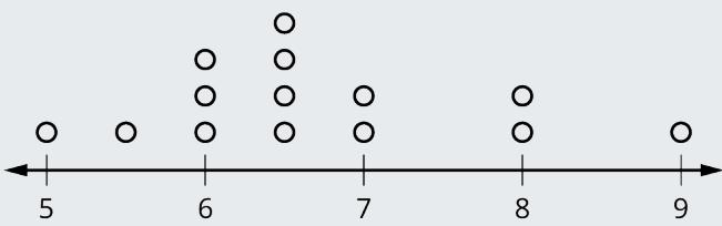
Figure 1.1.1 — A dot plot showing the frequency of the average time, in hours, that students reported sleeping per night. Each dot represents one student's response, stacked above its value on the number line.

Figure 1.1.1 — Frequency of average time (in hours) spent sleeping per night.

The questions above ask you to analyze and interpret your data. With this small example, you have already begun your study of statistics.

Here is the one-sentence version of the whole course: descriptive statistics describes the data you actually have, while inferential statistics uses that data to make a careful guess about a much larger group you could never measure all of. Describe first, then infer.

In this course, you will learn how to organize and summarize data. Organizing and summarizing data is called descriptive statistics. Two ways to summarize data are by graphing and by using numbers (for example, finding an average). After you have studied probability and probability distributions, you will use formal methods for drawing conclusions from "good" data. Those formal methods are called inferential statistics — and statistical inference uses probability to measure how confident we can be that our conclusions are correct.

Effective interpretation of data (inference) rests on two things: good procedures for producing data, and thoughtful examination of the data you produced. Along the way you will meet what can feel like too many formulas. But the goal of statistics is not to grind through calculations — a calculator or computer can do those. The goal is to understand your data, and that understanding has to come from you. If you genuinely grasp the basics, you can be far more confident in the decisions you make in life.

Try It Now 1.1.1

A researcher records the number of hours of sleep for every student in a single dorm and then makes a dot plot and computes the average. Later, she uses that average to estimate the typical nightly sleep of all students at the university.

Which part of her work is descriptive statistics, and which part is inferential statistics?

Solution

Descriptive statistics: making the dot plot and computing the average for the students in that one dorm. She is describing the data she actually collected.

Inferential statistics: using that average to estimate the typical sleep of all students at the university — a group far larger than the one she measured. She is inferring beyond her data.

Answer: the dot plot and average are descriptive; the university-wide estimate is inferential.

1.1.2 Probability

This "few tosses are wild, many tosses settle down" idea is the quiet engine behind everything to come. Insurance companies, casinos, and medical researchers cannot predict any single outcome — but over thousands of cases the long-run proportions become remarkably predictable. That predictability is exactly what probability lets us pin a number on.

Probability is a mathematical tool used to study randomness. It measures the chance (the likelihood) of an event occurring. For example, if you toss a fair coin four times, the outcome may not be exactly two heads and two tails. However, if you toss that same coin 4,000 times, the results will land close to half heads and half tails. The expected theoretical probability of heads on any single toss is \(\frac{1}{2}\), or \(0.5\). Even though the outcome of a few tosses is uncertain, a regular pattern emerges over many repetitions.

History backs this up. The English statistician Karl Pearson once tossed a coin 24,000 times and got 12,012 heads. One of the original authors tossed a coin 2,000 times and got 996 heads. The fraction \(\frac{996}{2000} = 0.498\) is very close to \(0.5\), the expected probability.

The theory of probability began with the study of games of chance, such as poker. Today, predictions of all kinds take the form of probabilities. To estimate the chance of an earthquake, of rain, or of getting an A in this course, we use probabilities. Doctors use probability to weigh the chance a vaccination causes the very disease it prevents. A stockbroker uses probability to estimate the rate of return on a client's investments. You might use probability to decide whether to buy a lottery ticket. Throughout your study of statistics, you will use the power of probability to analyze and interpret your data.

Try It Now 1.1.2

A weather service says there is a \(70\%\) chance of rain tomorrow. A friend objects: "It either rains or it doesn't — so the chance is really just 50/50." Explain why your friend is wrong, using what you know about how probability behaves over many repetitions.

Solution

Probability is not about a single yes/no outcome being "even." It is a long-run measure: of all the days the weather service has called "70% chance of rain" under similar conditions, rain has actually occurred on about \(70\%\) of them.

Saying "it rains or it doesn't, so 50/50" ignores all the information packed into the forecast. A fair coin is genuinely 50/50; tomorrow's weather, given the atmospheric data, is not.

Answer: the two outcomes (rain / no rain) are not equally likely, so the chance is \(70\%\), not \(50\%\). "Either/or" tells you the possible outcomes, not how likely each one is.

1.1.3 Populations, Samples, and Variables

Definition 1.1.1: Population

A population is the entire collection of persons, things, or objects under study. It is the whole group we ultimately want to draw a conclusion about.

Definition 1.1.2: Sample

A sample is a portion (a subset) of the population that we actually examine. We study the sample to gain information about the larger population. Data are the result of sampling from a population.

Definition 1.1.3: Statistic

A statistic is a number that represents a property of the sample — for example, the average score of the students in one class we surveyed. A statistic is an estimate of a population parameter.

A memory trick that pays off all term: the two p's go together, and the two s's go together. Parameter describes a Population; Statistic describes a Sample. Whenever you are unsure which word to use, check whether you are talking about the whole group (population → parameter) or just the part you measured (sample → statistic).

Definition 1.1.4: Parameter

A parameter is a numerical characteristic of the whole population — for example, the average score of every student in every class. We can rarely measure a parameter directly, so we estimate it with a statistic.

Definition 1.1.5: Variable

A variable, usually written with a capital letter such as \(X\) or \(Y\), is a characteristic or measurement that can be determined for each member of a population. Variables are either numerical (values with equal units, such as weight in pounds or time in hours) or categorical (values that place each member into a category).

Definition 1.1.6: Data

Data are the actual values of the variable. They may be numbers or words. A single value is called a datum.

We generally want to study a population — a collection of persons, things, or objects. Because examining an entire population usually costs too much time and money, we instead select a sample: a manageable subset that we study to learn about the whole. If you wanted the overall grade point average at your school, you would not track down every student — you would survey a sample, and the GPAs you collect would be your data. In presidential elections, opinion polls sample just 1,000–2,000 people yet aim to represent the views of an entire country. Manufacturers sample cans off the line to check whether a 16-ounce can really holds 16 ounces.

From the sample data we compute a statistic — a number summarizing the sample. The statistic estimates a parameter, the matching number for the whole population. One of the central concerns of statistics is how accurately a statistic estimates a parameter, and that accuracy depends on how well the sample represents the population. A good sample carries the characteristics of the population it came from. Figure 1.1.2 ties these four ideas together in one picture.
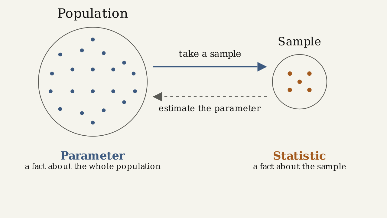
Figure 1.1.2 — A sample is drawn from a population; a statistic about the sample estimates a parameter about the whole population.

Figure 1.1.2 — A sample is drawn from a population; a statistic (about the sample) estimates a parameter (about the whole population).

A bit more vocabulary you will reach for constantly. To see how a variable works, suppose we let \(X\) equal the number of points earned by one math student at the end of a term; then \(X\) is a numerical variable. If instead we let \(Y\) be a person's party affiliation, then values of \(Y\) include Republican, Democrat, and Independent, so \(Y\) is a categorical variable. We can do arithmetic with the values of \(X\) (we can average points earned), but it makes no sense to do arithmetic with the values of \(Y\) (there is no "average party affiliation").

Two more words show up often: mean and proportion. If you scored 86, 75, and 92 on three exams, your mean score is \(\frac{86 + 75 + 92}{3} = 84.3\) (to one decimal place). A proportion is the fraction of a group with some characteristic. For instance, if your math class has 40 students and 18 of them are women, then the proportion of women students is \(\frac{18}{40} = 0.45\). Mean and proportion both get a much fuller treatment in later chapters.

The words "mean" and "average" are often used interchangeably, and that substitution is common practice. The precise technical term is arithmetic mean; "average" technically refers to a center location. Among non-statisticians, though, "average" is widely accepted as standing in for "arithmetic mean."

Try It Now 1.1.3

Determine what the key terms refer to in the following study. We want to know the average (mean) amount of money spent on school uniforms each year by families with children at Knoll Academy. We randomly survey 100 families with children in the school. Three of the families spent $65, $75, and $95, respectively.

Solution
  • Population: all families with children attending Knoll Academy.
  • Sample: the 100 families randomly surveyed.
  • Parameter: the average (mean) yearly amount spent on uniforms by all Knoll Academy families.
  • Statistic: the average (mean) yearly amount spent on uniforms by the 100 families in the sample.
  • Variable: \(X\) = the amount one surveyed family spends on uniforms in a year.
  • Data: the dollar amounts spent, such as $65, $75, and $95.
Example 1.1.1

Determine what the key terms refer to in the following study. We want to know the average (mean) amount of money first-year college students spend at ABC College on school supplies that do not include books. We randomly surveyed 100 first-year students at the college. Three of those students spent $150, $200, and $225, respectively.

Solution

Population: all first-year students attending ABC College this term.

Sample: the group we actually surveyed — for instance, all students enrolled in one section of a beginning statistics course at ABC College (note that such a sample may not perfectly represent the whole population).

Parameter: the average (mean) amount of money spent on supplies (excluding books) by all first-year students at ABC College this term.

Statistic: the average (mean) amount spent (excluding books) by the first-year students in the sample.

Variable: let \(X\) = the amount of money spent (excluding books) by one first-year student attending ABC College.

Data: the dollar amounts spent by the surveyed first-year students — for example, $150, $200, and $225.

Try It Now 1.1.4

Determine what the key terms refer to in the following study. A study was conducted at a local college to analyze the average cumulative GPA of students who graduated last year. Match the letter of the phrase that best describes each item.

  1. Population _____
  2. Statistic _____
  3. Parameter _____
  4. Sample _____
  5. Variable _____
  6. Data _____
  1. all students who attended the college last year
  2. the cumulative GPA of one student who graduated from the college last year
  3. 3.65, 2.80, 1.50, 3.90
  4. a group of students who graduated from the college last year, randomly selected
  5. the average cumulative GPA of students who graduated from the college last year
  6. all students who graduated from the college last year
  7. the average cumulative GPA of students in the study who graduated from the college last year
Solution
  1. Population → f (all students who graduated last year)
  2. Statistic → g (average GPA of the students in the study)
  3. Parameter → e (average GPA of all graduates)
  4. Sample → d (the randomly selected group of graduates)
  5. Variable → b (the GPA of one graduate)
  6. Data → c (the actual GPA values: 3.65, 2.80, 1.50, 3.90)

Answer: 1‑f, 2‑g, 3‑e, 4‑d, 5‑b, 6‑c.

Example 1.1.2

Determine what the key terms refer to in the following study. A survey of athletes at a university was conducted to study the heights of athletes, in meters. Match the letter of the phrase that best describes each item.

  1. Population
  2. Statistic
  3. Parameter
  4. Sample
  5. Variable
  6. Data
  1. the average height of athletes in the university
  2. the average height of athletes in the survey
  3. all athletes in the university
  4. all students in the university
  5. the height of one athlete
  6. a group of athletes randomly selected
  7. 1.82, 1.76, 1.69, 1.93
Solution
  1. Population → c (all athletes in the university — not d, which is all students)
  2. Statistic → b (average height of athletes in the survey)
  3. Parameter → a (average height of all athletes in the university)
  4. Sample → f (the randomly selected group of athletes)
  5. Variable → e (the height of one athlete)
  6. Data → g (the actual heights: 1.82, 1.76, 1.69, 1.93)

Answer: 1‑c, 2‑b, 3‑a, 4‑f, 5‑e, 6‑g.

Try It Now 1.1.5

Determine what the key terms refer to in the following study. A survey checks the time a mobile phone takes to charge its battery from 50% to 100%. The criteria used to collect the data are:

Table 1.1.1 — Charging-study criteria.
Wattage of charger usedType of mobile used
30 WAndroid

We want to know the proportion of Android mobiles that charge to 100% within 30 minutes. We start with a simple random sample of 200 mobiles.

Solution
  • Population: all Android mobiles (charged with a 30 W charger) that the study is about.
  • Sample: the 200 mobiles selected by simple random sampling.
  • Parameter: the proportion of all such Android mobiles that reach 100% within 30 minutes.
  • Statistic: the proportion of the 200 sampled mobiles that reach 100% within 30 minutes.
  • Variable: \(X\) = whether a given mobile reaches 100% within 30 minutes (yes or no).
  • Data: the yes/no results — yes, charged within 30 minutes, or no, did not.
Example 1.1.3

Determine what the key terms refer to in the following study. As part of a study designed to test the safety of electric automobiles, the National Transportation Safety Board collected and reviewed data about the effects of a crash on test dummies. Here is the criterion they used:

Table 1.1.2 — Crash-test criterion.
Speed at which cars crashedLocation of "drivers" (i.e., dummies)
35 miles/hourFront seat

Cars with dummies in the front seats were crashed into a wall at 35 miles per hour. We want to know the proportion of dummies in the driver's seat that would have had head injuries, had they been actual drivers. We start with a simple random sample of 75 cars.

Solution

Population: all cars containing dummies in the front seat.

Sample: the 75 cars selected by a simple random sample.

Parameter: the proportion of driver dummies (if they had been real people) who would have suffered head injuries, across the whole population.

Statistic: the proportion of driver dummies who would have suffered head injuries, within the sample of 75 cars.

Variable: \(X\) = whether a dummy (if it had been a real person) would have suffered a head injury.

Data: either yes, had a head injury or no, did not.

Try It Now 1.1.6

Determine what the key terms refer to in the following study. A news agency wants to find the proportion of all truck drivers who have no points on their license. The agency randomly selects 1,000 truck drivers from the directory of truck drivers and determines how many in the sample have no points.

Solution
  • Population: all truck drivers in the directory.
  • Sample: the 1,000 truck drivers randomly selected.
  • Parameter: the proportion of all truck drivers in the directory with no points on their license.
  • Statistic: the proportion of the 1,000 sampled drivers with no points.
  • Variable: \(X\) = whether a given truck driver has no points on their license (yes or no).
  • Data: the yes/no results for the sampled drivers.
Example 1.1.4

Determine what the key terms refer to in the following study. An insurance company wants to determine the proportion of all medical doctors who have been involved in one or more malpractice lawsuits. The company selects 500 doctors at random from a professional directory and determines how many in the sample have been involved in a malpractice lawsuit.

Solution

Population: all medical doctors listed in the professional directory.

Sample: the 500 doctors selected at random from the directory.

Parameter: the proportion of all listed doctors who have been involved in one or more malpractice suits.

Statistic: the proportion of the 500 sampled doctors who have been involved in one or more malpractice suits.

Variable: \(X\) = whether an individual doctor has been involved in a malpractice suit.

Data: either yes, was involved in one or more malpractice lawsuits or no, was not.

Work in groups of up to four. Find a population, a sample, the parameter, the statistic, a variable, and the data for the following study: you want to determine the average (mean) number of glasses of milk college students drink per day. Suppose yesterday, in your English class, you asked five students how many glasses of milk they drank the day before, and the answers were 1, 0, 1, 3, and 4 glasses of milk.

1.1.4 Types of Variables

We just saw that variables come in two broad flavors — numerical and categorical. Numerical variables split one step further. A discrete numerical variable comes from counting (whole-number results like the number of siblings), while a continuous numerical variable comes from measuring on a scale that can take any value in a range (like height, which can be 1.72 m or 1.7236 m). Categorical variables, by contrast, sort each individual into a group rather than attaching a number.

Try It Now 1.1.7

For each pair of variables, decide whether you would expect them to be associated or independent:

  1. A person's height and their shoe size.
  2. The last digit of a person's phone number and their favorite color.
Solution
  1. Associated — taller people tend to have larger feet, so knowing height gives you some information about shoe size.
  2. Independent — there is no reason the last digit of a phone number would tell you anything about a favorite color; knowing one gives no information about the other.

Answer: (a) associated; (b) independent.

To close the loop on vocabulary: we collect a sample of data to better understand a population. A variable is the characteristic we measure for each individual or case. The overall quantity of interest — the mean, the median, a proportion, or some other summary of the whole population — is a parameter. We estimate that parameter by taking a sample and computing a matching numerical summary, the statistic. Remember the mnemonic: the two p's (population, parameter) go together, and the two s's (sample, statistic) go together.

Example 1.1.5

Data were collected about students in a statistics course. Three variables were recorded for each student: number of siblings, student height, and whether the student had previously taken a statistics course. Classify each variable as continuous numerical, discrete numerical, or categorical.

Solution

Number of siblings — this is a count, and counts are whole numbers, so it is a discrete numerical variable.

Student height — height varies smoothly along a scale and can take any value in a range, so it is a continuous numerical variable.

Previously taken a statistics course? — this sorts each student into one of two groups (yes or no) rather than attaching a number, so it is a categorical variable.

Answer: siblings = discrete numerical; height = continuous numerical; prior course = categorical.

Associated or Independent, Not Both

A pair of variables are either related in some way (associated) or not (independent). No pair of variables is both associated and independent at the same time.

Problem Set 1.1

Try It Now 1.2.1

The data are the number of machines in a gym. You sample five gyms. One gym has 12 machines, one has 15, one has ten, one has 22, and the last has 20 machines. What type of data is this?

Solution

We counted machines, and you cannot have a fractional machine — the values are whole numbers.

Answer: quantitative discrete data.

Example 1.2.1: Data Sample of Quantitative Discrete Data

The data are the number of books students carry in their backpacks. You sample five students. Two students carry three books, one student carries four books, one student carries two books, and one student carries one book. The numbers of books — three, four, two, and one — are the data.

What type of data is this?

Solution

Step 1 — counting or measuring? We counted books. You cannot carry 2.5 books, so the values are whole numbers only.

Answer: quantitative discrete data.

Try It Now 1.2.2

The data are the areas of lawns in square feet. You sample five houses. The areas of the lawns are 144, 160, 190, 180, and 210 square feet. What type of data is this?

Solution

Area is measured, not counted, and could in principle take any value in a range.

Answer: quantitative continuous data.

Example 1.2.2: Data Sample of Quantitative Continuous Data

The data are the weights of backpacks with books in them. You sample the same five students. The weights (in pounds) of their backpacks are 6.2, 7, 6.8, 9.1, and 4.3. Notice that two backpacks carrying three books can still have different weights. What type of data is this?

Solution

Step 1 — counting or measuring? We measured weight on a scale, and weight can land at any value — 6.2, 6.8, and so on.

Answer: quantitative continuous data.

Try It Now 1.2.3

A purchasing manager bought the following materials for a company:

  • Two types of nails (2 kg box nails, 3 kg roofing nails)
  • One type of oil (4 L machine oil)
  • Four types of screws (3 kg wood screws, 5 kg machine screws, 1 kg set screws, 2 kg socket screws)

Name data sets that are quantitative discrete, quantitative continuous, and qualitative.

Solution
  • Quantitative discrete: the counts of each item — two types of nails, one type of oil, four types of screws.
  • Quantitative continuous: the weights and volumes — 2 kg, 3 kg, 4 L, 3 kg, 5 kg, 1 kg, 2 kg — because they are measured.
  • Qualitative: the kinds of materials — box nails, roofing nails, machine oil, wood screws, machine screws, set screws, socket screws.
Example 1.2.3: Sorting a Shopping Trip

You go to the supermarket and buy three cans of soup (19-ounce tomato bisque, 14.1-ounce lentil, and 19-ounce Italian wedding), two packages of nuts (walnuts and peanuts), four kinds of vegetable (broccoli, cauliflower, spinach, and carrots), and two desserts (16-ounce pistachio ice cream and 32-ounce chocolate chip cookies).

Name data sets that are quantitative discrete, quantitative continuous, and qualitative.

Solution

One possible solution:

  • Quantitative discrete: the three cans of soup, two packages of nuts, four kinds of vegetables, and two desserts — because you count them.
  • Quantitative continuous: the weights of the soups (19 ounces, 14.1 ounces, 19 ounces) — because you measure weight as precisely as possible.
  • Qualitative: the types of soups, nuts, vegetables, and desserts — because they are categories.

Try to identify additional data sets in this example on your own.

Try It Now 1.2.4

The data are the colors of houses. You sample five houses. The colors are white, yellow, white, red, and white. What type of data is this?

Solution

The values are color names — categories, not numbers.

Answer: qualitative (categorical) data.

Example 1.2.4: Data Sample of Qualitative Data

The data are the colors of backpacks. Again, you sample the same five students. One student has a red backpack, two have black backpacks, one has a green backpack, and one has a gray backpack. The colors red, black, black, green, and gray are the data. What type of data is this?

Solution

The values are color names, not numbers, and averaging colors is nonsense.

Answer: qualitative (categorical) data.

Try It Now 1.2.5

Determine the correct data type for the number of cars in a parking lot. If it is quantitative, say whether it is continuous or discrete.

Solution

We count cars, and the values are whole numbers.

Answer: quantitative discrete data.

Example 1.2.5: Classify Each by Type

Work collaboratively to determine the correct data type (quantitative or qualitative). For quantitative data, also say whether it is continuous or discrete. Hint: data that are discrete often start with the words "the number of."

  1. the number of pairs of shoes you own
  2. the type of car you drive
  3. the distance from your home to the nearest grocery store
  4. the number of classes you take per school year
  5. the type of calculator you use
  6. weights of dogs at an animal shelter
  7. number of correct answers on a quiz
  8. IQ scores (this may cause some discussion)
Solution
  • Quantitative discrete (counted): a, d, and g.
  • Quantitative continuous (measured): c, f, and h.
  • Qualitative (categorical): b and e.
Try It Now 1.2.6

The registrar at State University keeps records of the number of credit hours students complete each semester, summarized in the histogram in Figure 1.2.1. The class boundaries are 10 to less than 13, 13 to less than 16, 16 to less than 19, 19 to less than 22, and 22 to less than 25. What type of data does this graph show?
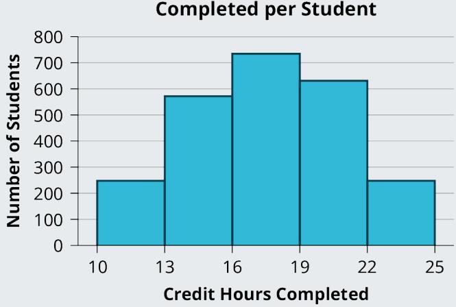
Figure 1.2.1 — Histogram titled

Solution

Credit hours are measured on a scale and grouped into intervals — the histogram is built for continuous data.

Answer: quantitative continuous data.

Example 1.2.6: Reading Data Off a Graph

A statistics professor records each student's classification — first-year student, sophomore, junior, or senior — and summarizes it in the pie chart in Figure 1.2.2. What type of data does this graph show?
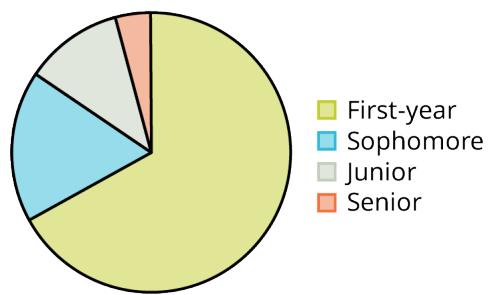
Figure 1.2.2 — Pie chart titled

Solution

The categories are years in school — first-year, sophomore, junior, senior. These are groups, not numbers you would average.

Answer: qualitative (categorical) data.

Try It Now 1.2.7

A survey reports the percent of students at a college who play each of several intramural sports, and a single student is allowed to sign up for more than one sport. The reported percentages add up to 130%. Should this be displayed as a pie chart or a bar graph? Why?

Solution

Because a student can be in more than one category, the percentages add to more than 100%. A pie chart's wedges must total exactly 100%, so a pie chart cannot represent this data honestly.

Answer: use a bar graph, not a pie chart.

Try It Now 1.2.8

Determine the type of sampling used (simple random, stratified, systematic, cluster, or convenience): a high school principal polls 50 first-year students, 50 sophomores, 50 juniors, and 50 seniors regarding policy changes for after-school activities.

Solution

The population is divided into groups (the four grade levels), and a sample is taken from each group.

Answer: stratified sampling.

Try It Now 1.2.9

A pharmaceutical company runs and pays for a study concluding that its own new drug is highly effective, and the study surveys only patients who chose to stay enrolled to the end. Name two of the critical-evaluation problems above that this scenario raises.

Solution
  • Self-funded / self-interest study: the company stands to gain from a favorable result, so the study may not be impartial — read it carefully on its merits.
  • Non-response / self-selection: surveying only patients who chose to stay enrolled drops anyone who quit (perhaps because the drug did not work or caused side effects), so the remaining responses may overstate effectiveness.

Answer: self-funded/self-interest bias and non-response (self-selection) bias.

Example 1.2.7: Identify the Sampling Method

A study determines the average tuition that San Jose State undergraduates pay per semester. Each student in the samples below is asked how much tuition they paid for the Fall semester. What is the type of sampling in each case?

  1. A sample of 100 undergraduates is taken by organizing students' names by classification (first-year, sophomore, junior, senior) and then selecting 25 students from each group.
  2. A random number generator selects one student from the alphabetical list of all undergraduates. Starting there, every 50th student is chosen until 75 students are included.
  3. A completely random method selects 75 students; each undergraduate has the same probability of being chosen at any stage.
  4. The first-year, sophomore, junior, and senior classes are numbered 1, 2, 3, 4. A random number generator picks two of those years, and all students in those two years are in the sample.
  5. An administrative assistant stands in front of the library one Wednesday and asks the first 100 undergraduates he meets what they paid in tuition.
Solution
  • a. stratified — split into groups (years) and sampled within each.
  • b. systematic — random start, then every 50th student.
  • c. simple random — every student equally likely at every stage.
  • d. cluster — picked whole groups (two years) and took everyone in them.
  • e. convenience — whoever happened to be there.

Answer: a. stratified; b. systematic; c. simple random; d. cluster; e. convenience.

Try It Now 1.2.10

You will use a random number generator to draw different types of samples from the quiz-score data below. The table shows six sets of quiz scores (each quiz is worth 10 points) for an elementary statistics class.

Table 1.2.5 — Six columns of quiz scores (out of 10).
#1#2#3#4#5#6
5710983
1059876
9108679
91010989
789574
9991087
7710988
8891088
978778
8810987

Use the random number generator to pick samples:

  1. Stratified sample by column. Pick three quiz scores randomly from each column. Number each row 1 through 10. On your calculator, press MATH, arrow to PRB, press 5:randInt(, enter 1,10), and press ENTER. Record the number, press ENTER twice more (even repeats), and record those numbers. Record the three quiz scores in that column matching the three row numbers. Repeat for columns 2 through 6. These 18 scores are a stratified sample.
  2. Cluster sample. Pick two of the columns. Press MATH, arrow to PRB, press 5:randInt(, enter 1,6), press ENTER, record the number, press ENTER again, and record that number. The quiz scores (20 of them) in those two columns are the cluster sample.
  3. Simple random sample of 15 scores. Number the scores 1 through 60. Press MATH, arrow to PRB, press 5:randInt(, enter 1, 60). Press ENTER 15 times and record the numbers. Record the matching quiz scores. These 15 scores are the simple random sample.
  4. Systematic sample of 12 scores. Number the scores 1 through 60. Press MATH, arrow to PRB, press 5:randInt(, enter 1, 60), press ENTER, and record the number and its quiz score. From that number, count ten scores and record that score; keep counting ten and recording until you have 12 scores. You may wrap around to the beginning.
Solution

This is a hands-on calculator activity, so answers depend on the random numbers your calculator produces. The point is the method, not a single right list:

  • Stratified: three scores per column gives \(3 \times 6 = 18\) scores.
  • Cluster: two whole columns gives \(2 \times 10 = 20\) scores.
  • Simple random: 15 scores drawn from the full pool of 60.
  • Systematic: a random start, then every tenth score, for 12 scores.

Each method should pull from the table as described above.

Example 1.2.8: Identify the Sampling Method Again

Determine the type of sampling used (simple random, stratified, systematic, cluster, or convenience).

  1. A soccer coach selects six players from boys aged 8–10, seven from boys aged 11–12, and three from boys aged 13–14 to form a team.
  2. A pollster interviews all human-resource personnel in five different high-tech companies.
  3. An education researcher interviews 50 public high school teachers and 50 private high school teachers.
  4. A medical researcher interviews every third cancer patient from a list of cancer patients at a local hospital.
  5. A high school counselor uses a computer to generate 50 random numbers and picks the students whose names match those numbers.
  6. A student interviews classmates in their algebra class to find the average number of pairs of jeans a student owns.
Solution
  • a. stratified — sampled within each age group.
  • b. cluster — picked whole groups (companies) and took everyone in them.
  • c. stratified — sampled within each group (public, private).
  • d. systematic — every third patient on the list.
  • e. simple random — computer-generated random selection.
  • f. convenience — whoever was in their own class.

Answer: a. stratified; b. cluster; c. stratified; d. systematic; e. simple random; f. convenience.

Try It Now 1.2.11

A local radio station has a fan base of 20,000 listeners and wants to know whether its audience prefers more music or more talk shows. Asking all 20,000 is nearly impossible, so the station uses convenience sampling and surveys the first 200 people it meets at one of its music concert events. Of those, 24 prefer more talk shows and 176 prefer more music. Is this sample representative of the entire 20,000-listener population?

Solution

No. The sample was gathered at a music concert, so it over-represents people who already like music — exactly the preference being measured. People who would rather hear talk shows are unlikely to be at a music event, so they are under-represented. This is a biased convenience sample.

Answer: the sample is not representative; it is biased toward music fans.

Example 1.2.9: When a Sample Misrepresents the Population

Suppose ABC College has 10,000 part-time students (the population), and we want the average amount a part-time student spends on books in the fall term. Asking all 10,000 students is nearly impossible, so we take samples.

First, we use convenience sampling and survey ten students from a first-term organic chemistry class. Many also take first-term calculus. They spend:

$128; $87; $173; $116; $130; $204; $147; $189; $93; $153

Second, using a list of senior citizens who take P.E. classes, we take every fifth senior citizen, for ten people. They spend:

$50; $40; $36; $15; $50; $100; $40; $53; $22; $22

It is unlikely any student is in both samples.

  1. Is either sample representative of the entire 10,000 part-time student population?
  2. Since these samples are not representative, is it wise to use them to describe the whole population?
  3. Now suppose we take a third sample: ten part-time students, one chosen by simple random sampling from each of ten disciplines (chemistry, math, English, psychology, sociology, history, nursing, physical education, art, and early childhood development), assuming equal enrollment across disciplines. They spend:

$180; $50; $150; $85; $260; $75; $180; $200; $200; $150

Is this third sample biased?

Solution

a. No. The first sample is mostly science-oriented students whose books (chemistry, calculus) tend to be expensive, so they likely pay more than the average part-time student. The second sample is senior citizens taking courses for health and interest, who likely pay less. Both are biased, and in both cases not all students had a chance to be chosen.

b. No. In these samples, each member of the population did not have an equally likely chance of being chosen, so the results should not be used to describe the whole population.

c. The third sample is unbiased, but a larger sample would be recommended to increase the chance that it closely represents the population. (For a biased technique, even a large sample risks being unrepresentative.) Students often ask whether sampling is "good enough" instead of surveying everyone. If the survey is done well, the answer is yes.

Try It Now 1.2.12

Two students each take a random sample of 40 classmates and compute the average height. They get slightly different averages. Does this mean one of them made a mistake?

Solution

No. Two random samples from the same population almost never produce identical results — that is normal sampling variation, not an error. Neither student is wrong; their averages simply reflect two different subsets of the same population.

Answer: no mistake — this is ordinary variation between samples.

Try It Now 1.2.13

A pollster says a national survey of 1,500 randomly chosen, well-surveyed adults is "large enough" to be reliable, but a call-in survey with 50,000 responses is not. How can the smaller sample be more trustworthy than the bigger one?

Solution

Sheer size does not fix bias. The call-in survey is self-selected — only people motivated to call in respond — so even 50,000 responses can be wildly unrepresentative. The 1,500-person survey is random, so every adult had an equal chance of being chosen, which keeps it representative. A smaller unbiased sample beats a huge biased one.

Answer: the 1,500-person random survey is more reliable because it is unbiased; the call-in survey, despite its size, is biased by self-selection.

Studies are often done by pharmaceutical companies to determine the effectiveness of a treatment program. Suppose that a new drug is currently under study to address a respiratory virus. It is given to patients once the patient exhibits symptoms of the virus. Of interest is the average (mean) length of time in days from the time the patient starts the treatment until the symptoms are alleviated. Two researchers each follow a different set of 40 patients with the respiratory virus from the start of treatment until the symptoms are alleviated. The following data (in days) are collected.

Researcher A: 3; 4; 11; 15; 16; 17; 22; 44; 37; 16; 14; 24; 25; 15; 26; 27; 33; 29; 35; 44; 13; 21; 22; 10; 12; 8; 40; 32; 26; 27; 31; 34; 29; 17; 8; 24; 18; 47; 33; 34

Researcher B: 3; 14; 11; 5; 16; 17; 28; 41; 31; 18; 14; 14; 26; 25; 21; 22; 31; 2; 35; 44; 23; 21; 21; 16; 12; 18; 41; 22; 16; 25; 33; 34; 29; 13; 18; 24; 23; 42; 33; 29

For problems 1 through 5, determine what the key terms refer to in the example for Researcher A.

Problem 1. population

Solution

Step 1 — Recall the definition: The population is the entire collection of individuals or objects we want to draw a conclusion about.

Step 2 — Apply it to Researcher A's study: The goal is to learn about the recovery time for all patients who take the new drug for this respiratory virus, not just the 40 who were followed.

Answer: The population is all patients with the respiratory virus who take the new drug (every person to whom the treatment could apply).

Problem 2. sample

Solution

Step 1 — Recall the definition: A sample is the subset of the population that is actually observed and measured.

Step 2 — Apply it to Researcher A's study: Researcher A did not measure every drug-taking patient — only the specific 40 patients he followed from treatment start to relief.

Answer: The sample is the 40 patients with the respiratory virus that Researcher A followed.

Problem 3. parameter

Solution

Step 1 — Recall the definition: A parameter is a numerical summary that describes a characteristic of the entire population.

Step 2 — Apply it to Researcher A's study: The quantity of interest is the average recovery time. Computed over the whole population, that mean is a parameter.

Answer: The parameter is the (unknown) mean number of days to symptom relief for the entire population of patients taking the drug.

Problem 4. statistic

Solution

Step 1 — Recall the definition: A statistic is a numerical summary computed from the sample; it estimates the corresponding parameter.

Step 2 — Apply it to Researcher A's study: The mean recovery time calculated from Researcher A's 40 patients is a statistic.

Answer: The statistic is the mean number of days to symptom relief computed from Researcher A's sample of 40 patients.

Problem 5. variable

Solution

Step 1 — Recall the definition: A variable is the characteristic being measured on each member of the sample; its value changes from patient to patient.

Step 2 — Apply it to Researcher A's study: The measured characteristic is the length of time, in days, from the start of treatment until symptoms are relieved.

Answer: The variable is \(X =\) the number of days from the start of treatment until the patient's symptoms are alleviated.

For each of problems 6 through 13, identify: a) the population, b) the sample, c) the parameter, d) the statistic, e) the variable, and f) the data. Give examples where appropriate.

Problem 6. A fitness center is interested in the mean amount of time a client exercises in the center each week.

Solution

Step 1 — Apply the definitions: Population = the entire group of interest; sample = the subset actually studied; parameter = a numerical fact about the population; statistic = a numerical fact computed from the sample; variable = the characteristic being measured; data = the actual values recorded.

Step 2 — Map them to this scenario (mean weekly exercise time):

a) Population: all clients of the fitness center.

b) Sample: the particular group of clients whose exercise time is actually measured.

c) Parameter: the mean weekly exercise time of all clients.

d) Statistic: the mean weekly exercise time of the sampled clients.

e) Variable: \(X =\) the amount of time (e.g., hours) a client exercises in the center per week.

f) Data: the individual recorded times, e.g., 2 hours, 5 hours, 3.5 hours, ….

Answer: a) all fitness-center clients; b) the clients actually surveyed; c) mean weekly exercise time of all clients; d) mean weekly exercise time of the sampled clients; e) weekly exercise time per client; f) the specific time values recorded (e.g., 2, 5, 3.5 hours).

Problem 7. Ski resorts are interested in the mean age that children take their first ski and snowboard lessons. They need this information to plan their ski classes optimally.

Solution

Step 1 — Recall the six definitions: population (whole group), sample (subset studied), parameter (population number), statistic (sample number), variable (measured characteristic), data (the recorded values).

Step 2 — Map them to this scenario (mean age of first ski/snowboard lesson):

a) Population: all children who take ski and snowboard lessons (at the resorts of interest).

b) Sample: the particular group of children whose first-lesson ages are recorded.

c) Parameter: the mean first-lesson age of all such children.

d) Statistic: the mean first-lesson age of the sampled children.

e) Variable: \(X =\) the age at which a child takes their first ski/snowboard lesson.

f) Data: the individual ages, e.g., 4 years, 6 years, 5 years, ….

Answer: a) all children taking ski/snowboard lessons; b) the children actually surveyed; c) mean first-lesson age of all such children; d) mean first-lesson age of the sample; e) age at first lesson; f) the specific ages recorded (e.g., 4, 6, 5 years).

Problem 8. A cardiologist is interested in the mean recovery period of their patients who have had heart attacks.

Solution

Step 1 — Recall the six definitions: population, sample, parameter (population number), statistic (sample number), variable (measured trait), data (recorded values).

Step 2 — Map them to this scenario (mean recovery period after heart attack):

a) Population: all of the cardiologist's patients who have had heart attacks.

b) Sample: the particular group of those patients whose recovery time is measured.

c) Parameter: the mean recovery period of all the cardiologist's heart-attack patients.

d) Statistic: the mean recovery period of the sampled patients.

e) Variable: \(X =\) the length of the recovery period (e.g., in days) for a heart-attack patient.

f) Data: the individual recovery times, e.g., 30 days, 45 days, 28 days, ….

Answer: a) all of the cardiologist's heart-attack patients; b) the patients actually measured; c) mean recovery period of all such patients; d) mean recovery period of the sample; e) recovery-period length per patient; f) the specific recovery times recorded (e.g., 30, 45, 28 days).

Problem 9. Insurance companies are interested in the mean health costs each year of their clients, so that they can determine the costs of health insurance.

Solution

Step 1 — Recall the six definitions: population, sample, parameter (population number), statistic (sample number), variable (measured trait), data (recorded values).

Step 2 — Map them to this scenario (mean annual health costs of clients):

a) Population: all clients of the insurance company.

b) Sample: the particular group of clients whose annual health costs are examined.

c) Parameter: the mean annual health cost of all clients.

d) Statistic: the mean annual health cost of the sampled clients.

e) Variable: \(X =\) the annual health cost of a client (in dollars).

f) Data: the individual cost values, e.g., $2,000, $5,500, $1,200, ….

Answer: a) all clients of the insurance company; b) the clients actually sampled; c) mean annual health cost of all clients; d) mean annual health cost of the sample; e) annual health cost per client; f) the specific cost values recorded (e.g., $2,000, $5,500, $1,200).

Problem 10. A politician is interested in the proportion of voters in their district who think the politician is doing a good job.

Solution

Step 1 — Recall the six definitions: population, sample, parameter (population number), statistic (sample number), variable (measured trait), data (recorded values).

Step 2 — Map them to this scenario (proportion of voters who approve):

a) Population: all voters in the politician's district.

b) Sample: the particular group of voters who are actually surveyed.

c) Parameter: the proportion of all district voters who think the politician is doing a good job.

d) Statistic: the proportion of the sampled voters who think so.

e) Variable: \(X =\) whether a given voter thinks the politician is doing a good job (yes/no).

f) Data: the individual yes/no responses, e.g., yes, no, yes, yes, no, ….

Answer: a) all voters in the district; b) the voters actually surveyed; c) the true proportion of all district voters who approve; d) the proportion of surveyed voters who approve; e) each voter's approval (yes/no); f) the specific yes/no responses recorded.

Problem 11. A marriage counselor is interested in the proportion of clients they counsel who stay married.

Solution

Step 1 — Identify the population: The population is the entire group the counselor wants to draw conclusions about — here, all of the counselor's clients (those they counsel).

Step 2 — Identify the parameter of interest: The proportion of all clients who stay married. This is the population proportion, the numerical fact the counselor wants to learn.

Step 3 — Identify the variable and data: The variable is whether a given client stays married (yes/no). The data are the actual yes/no responses recorded for the clients studied.

Answer: Population = all clients the counselor counsels; parameter = the (true) proportion of those clients who stay married; variable = whether a client stays married; data = the yes/no marital-status outcomes collected.

Problem 12. Political pollsters may be interested in the proportion of people who will vote for a particular cause.

Solution

Step 1 — Identify the population: The population is everyone whose vote the pollsters care about — all eligible voters (the people who could vote on the cause).

Step 2 — Identify the parameter of interest: The proportion of all those people who will vote for the particular cause. This is the population proportion.

Step 3 — Identify the variable and data: The variable is whether a given person will vote for the cause (yes/no). The data are the recorded yes/no voting intentions.

Answer: Population = all eligible voters; parameter = the proportion who will vote for the cause; variable = whether a person votes for the cause; data = the yes/no responses collected.

Problem 13. A marketing company is interested in the proportion of people who will buy a particular product.

Solution

Step 1 — Identify the population: The population is all the people the marketing company is interested in — the potential buyers of the product.

Step 2 — Identify the parameter of interest: The proportion of all those people who will buy the particular product. This is the population proportion.

Step 3 — Identify the variable and data: The variable is whether a given person will buy the product (yes/no). The data are the recorded yes/no purchase responses.

Answer: Population = all potential buyers (people the company is interested in); parameter = the proportion who will buy the product; variable = whether a person buys the product; data = the yes/no purchase outcomes collected.

For problems 14 through 16, a Lake Tahoe Community College instructor is interested in the mean number of days Lake Tahoe Community College math students are absent from class during a quarter.

Problem 14. What is the population she is interested in?

a) all Lake Tahoe Community College students

b) all Lake Tahoe Community College English students

c) all Lake Tahoe Community College students in her classes

d) all Lake Tahoe Community College math students

Solution

Step 1 — Read the question carefully: The instructor studies the mean days absent of math students, so the population must be exactly the group she wants conclusions about.

Step 2 — Eliminate options that are too broad or wrong: "All Lake Tahoe Community College students" (a) and "English students" (b) are not her group; "students in her classes" (c) is only a subset she might sample, not the full target group.

Step 3 — Select the matching group: The full target group is all Lake Tahoe Community College math students.

Answer: d) all Lake Tahoe Community College math students.

Problem 15. Consider the following: \(X\) = number of days a Lake Tahoe Community College math student is absent. In this case, \(X\) is an example of a:

a) variable.

b) population.

c) statistic.

d) data.

Solution

Step 1 — Recognize what \(X\) measures: \(X\) = the number of days a math student is absent. Its value changes from student to student, so it is a characteristic that varies across individuals.

Step 2 — Match to the term: A characteristic that takes different values for different members of the population is a variable. It is not the population (the students themselves), not a statistic (a single computed summary), and not the data (the actual recorded values).

Answer: a) variable.

Problem 16. The instructor's sample produces a mean number of days absent of 3.5 days. This value is an example of a:

a) parameter.

b) data.

c) statistic.

d) variable.

Solution

Step 1 — Identify the source of the number: The value 3.5 days is the mean computed from the instructor's sample, not from the entire population of math students.

Step 2 — Match to the term: A numerical summary computed from a sample is a statistic. (A parameter would summarize the whole population; data are the raw values; a variable is the characteristic measured.)

Answer: c) statistic.

Key Terms

statistics — the science of collecting, analyzing, interpreting, and presenting data.

descriptive statistics — organizing and summarizing data, for example with a graph or an average.

inferential statistics — using sample data, together with probability, to draw conclusions about a larger population.

probability — a mathematical measure of the chance that an event occurs; stable over many repetitions.

population — the entire collection of persons, things, or objects under study.

sample — a subset of the population that is actually examined.

parameter — a numerical characteristic of the whole population (e.g., a population mean).

statistic — a numerical summary of a sample, used to estimate a parameter.

variable — a characteristic or measurement recorded for each member of a population, usually written \(X\) or \(Y\).

numerical variable — a variable whose values are numbers with equal units (e.g., weight, time).

categorical variable — a variable that places each member into a category (e.g., party affiliation).

discrete variable — a numerical variable that comes from counting (whole-number values).

continuous variable — a numerical variable that comes from measuring on a scale (any value in a range).

data — the actual recorded values of a variable; a single value is a datum.

mean — the arithmetic average of a set of numerical values.

proportion — the fraction of a group that has a given characteristic.

associated / independent — two variables are associated if knowing one gives information about the other, and independent if it does not; no pair is both.

1.2 Data, Sampling, and Variation in Data and Sampling

Learning Objectives

In this section, you will learn to:
  • Sort data into qualitative (categorical) and quantitative (numerical) types.
  • Tell quantitative discrete data (from counting) apart from quantitative continuous data (from measuring).
  • Read and choose between pie charts, bar graphs, and Pareto charts for qualitative data.
  • Describe the main random sampling methods: simple random, stratified, cluster, and systematic.
  • Recognize convenience sampling, sampling bias, and the difference between sampling and nonsampling errors.
  • Explain why two samples from the same population vary, and why bigger (unbiased) samples are better.

In §1.1 we pinned down the vocabulary — population, sample, parameter, statistic, variable, data. Now we put that vocabulary to work. First we sort the data itself into types, because the type of data decides which graphs and which math even make sense. Then we look at how to actually get a sample that fairly represents a population, and we close by facing a fact of life in statistics: no two samples are ever exactly alike.

1.2.1 Kinds of Data

Definition 1.2.1: Qualitative Data

Qualitative data (also called categorical data) are the result of categorizing or describing attributes of a population. They are generally described by words or letters rather than numbers.

Hair color, blood type, ethnic group, the car a person drives, and the street a person lives on are all qualitative. Hair color might be black, dark brown, light brown, blonde, gray, or red; blood type might be AB+, O−, or B+. Researchers often prefer quantitative data because numbers lend themselves to mathematical analysis — it simply does not make sense to find an average hair color or an average blood type.

Definition 1.2.2: Quantitative Data

Quantitative data are always numbers. They are the result of counting or measuring attributes of a population.

Amount of money, pulse rate, weight, the number of people living in your town, and the number of students who take statistics are all quantitative. Quantitative data split one level further, into discrete and continuous.

Definition 1.2.3: Quantitative Discrete Data

Quantitative discrete data are the result of counting. They take on only certain numerical values — usually whole numbers.

If you count the number of phone calls you receive on each day of the week, you might get values such as 0, 1, 2, or 3. You will never get 2.5 phone calls, so the data are discrete.

Definition 1.2.4: Quantitative Continuous Data

Quantitative continuous data are the result of measuring. They are not limited to counting numbers — they may include fractions, decimals, or irrational numbers.

Continuous data usually come from measurements like lengths, weights, or times. A list of the lengths in minutes of all the phone calls you make in a week — numbers like 2.4, 7.5, or 11.0 — would be quantitative continuous data.

Why fuss over discrete versus continuous? Because it changes the math downstream. Discrete data are natural to display as counts and whole-number bars; continuous data get grouped into intervals and graphed as histograms. Tagging the data type now saves you from picking the wrong graph or the wrong formula three chapters from now. The examples below walk through each type one at a time so the distinction sticks before you have to choose a tool under pressure.

Data may come from a population or from a sample. We usually write data values with lowercase letters like \(x\) or \(y\). Almost every piece of data you will ever meet falls into one of two big buckets:

  • Qualitative (categorical)
  • Quantitative (numerical)

A student's backpack filled with textbooks; the count of books is quantitative discrete data.

A backpack on a scale; weight is measured, so it is quantitative continuous data.

A bag of groceries; the same shopping trip mixes discrete counts, continuous weights, and qualitative categories.

You may collect data as numbers and then report it categorically. For example, quiz scores are recorded as numbers throughout the term, but at the end the scores are reported as A, B, C, D, or F. The reporting form (letter grades) is qualitative even though the raw data were quantitative.

Backpacks of different colors; color is a category, so the data are qualitative.

A row of cars; the type of car you drive is qualitative data.

1.2.2 Displaying Qualitative Data

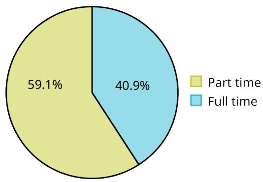
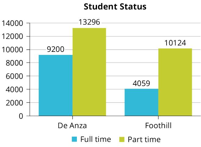
Once data are sorted by type, the next job is to show them. We start with qualitative data. Below are tables comparing the number of part-time and full-time students at De Anza College and Foothill College for the most recent spring quarter. The tables show counts (frequencies) and percentages or proportions (relative frequencies).

The percent columns make it easy to compare the same category across the two colleges. Showing percentages alongside the raw counts is always helpful, but it matters most when the totals differ — as they do here, since the two colleges have very different total enrollments. Notice how much larger the part-time percentage is at Foothill College than at De Anza College.

Table 1.2.1 — Full-time and part-time enrollment, most recent spring quarter.
StatusDe Anza — NumberDe Anza — PercentFoothill — NumberFoothill — Percent
Full-time9,20040.9%4,05928.6%
Part-time13,29659.1%10,12471.4%
Total22,496100%14,183100%

Tables are a good way to organize and display data, but graphs can make the patterns even easier to see. There are no strict rules about which graph to use. Three graphs are commonly used for qualitative data:

Pie Charts

In a pie chart, categories of data are shown as wedges of a circle, and each wedge is sized in proportion to the percent of individuals in that category.

Bar Graphs

In a bar graph, the length of each bar is proportional to the number or percent of individuals in that category. Bars may run vertically or horizontally.

Pareto Charts

A Pareto chart is a bar graph whose bars are sorted by category size, from largest to smallest. Sorting makes the biggest categories jump out immediately.

Look at the pie charts in Figure 1.2.3 and the bar graph in Figure 1.2.4 and decide which one you think shows the comparison better. It is a good idea to look at several graphs and pick whichever is most helpful for the data and the context — and that choice also depends on what you are using the data for.

Figure 1.2.3 — Side-by-side pie charts of full-time vs. part-time enrollment at De Anza College and Foothill College.

Figure 1.2.4 — Bar graph comparing full-time and part-time enrollment percentages at De Anza and Foothill Colleges.

When Percentages Add to More or Less Than 100%

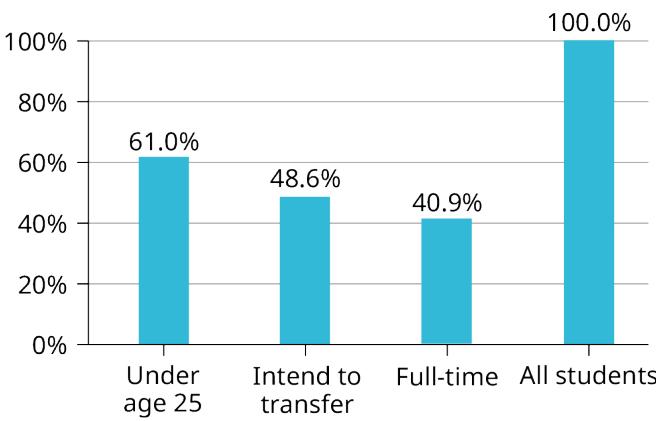
Sometimes the percentages add up to more than 100% (or less than 100%). In the data below, the percentages add to more than 100% because a student can fall into more than one category at once. When that happens, a bar graph is the right tool to compare the relative sizes of the categories — a pie chart cannot be used, because pie wedges must add to exactly 100%. (A pie chart also fails when the percentages add to less than 100%.)

Table 1.2.2 — De Anza College characteristics, most recent spring quarter (categories overlap, so percentages exceed 100%).
Characteristic / CategoryPercent
Full-Time Students40.9%
Students who intend to transfer to a 4-year institution48.6%
Students under age 2561.0%
Total150.5%

Figure 1.2.5 — Bar graph of overlapping De Anza student characteristics, whose percentages sum to more than 100%.

When a Category Is Missing

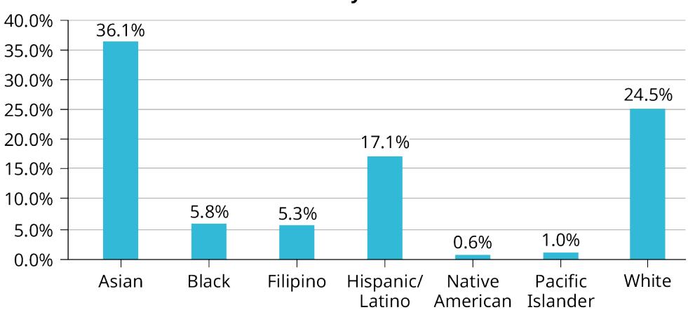
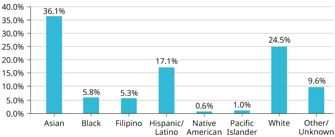
The next table displays the ethnicity of students but leaves out the "Other/Unknown" category — people who did not feel they fit any listed category or who declined to respond. Notice that the frequencies do not add up to the total number of students. In this situation, use a bar graph, not a pie chart, because the parts no longer make a whole.

Table 1.2.3 — Ethnicity of students at De Anza College, most recent fall term (Other/Unknown omitted).
EthnicityFrequencyPercent
Asian8,79436.1%
Black1,4125.8%
Filipino1,2985.3%
Hispanic/Latino4,18017.1%
Native American1460.6%
Pacific Islander2361.0%
White5,97824.5%
Total22,044 out of 24,38290.4% out of 100%

Figure 1.2.6 — Bar graph of student ethnicity at De Anza College with the Other/Unknown category omitted.

The next graph is the same as the one above, but now the "Other/Unknown" percent (9.6%) has been put back in. That category turns out to be large compared with some others (Native American at 0.6%, Pacific Islander at 1.0%), which is important to know when we think about what the data are telling us.

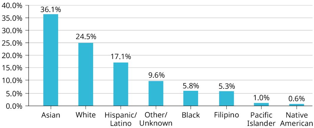
The bar graph in Figure 1.2.7 can be hard to read visually. The Pareto chart in Figure 1.2.8 fixes that: its bars are sorted from largest to smallest, so it is much easier to read and interpret.

Figure 1.2.7 — Bar graph of student ethnicity including the Other/Unknown category, in alphabetical order.

Figure 1.2.8 — Pareto chart of student ethnicity with bars sorted from largest to smallest.

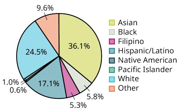
When the percentages do add to 100% (Other/Unknown included), a pie chart works again. The pie chart in Figure 1.2.9(b) is organized by wedge size, which makes it more informative than the unsorted, alphabetical version in Figure 1.2.9(a).

Figure 1.2.9 — Two pie charts of student ethnicity (Other/Unknown included): (a) alphabetical order, (b) sorted by wedge size.

1.2.3 Sampling Methods

Definition 1.2.5: Simple Random Sample

In a simple random sample, any group of individuals is equally likely to be chosen as any other group of the same size. In other words, every possible sample of a given size has an equal chance of being selected.

Suppose Lisa wants to form a four-person study group (herself plus three others) from her pre-calculus class, which has 31 other members. To choose a simple random sample of size three, Lisa could write all 31 names on slips, put them in a hat, shake it, close her eyes, and pick three. A more technological route is to list everyone's last name beside a two-digit ID, as in Table 1.2.4:

Table 1.2.4 — Class roster with two-digit IDs.
IDNameIDNameIDName
00Anselmo11King21Roquero
01Bautista12Legeny22Roth
02Bayani13Lundquist23Rowell
03Cheng14Macierz24Salangsang
04Cuarismo15Motogawa25Slade
05Cuningham16Okimoto26Stratcher
06Fontecha17Patel27Tallai
07Hong18Price28Tran
08Hoobler19Quizon29Wai
09Jiao20Reyes30Wood
10Khan

Lisa can use a table of random numbers, a calculator, or a computer to generate random numbers. Suppose her calculator produces:

0.94360; 0.99832; 0.14669; 0.51470; 0.40581; 0.73381; 0.04399

She reads each value in two-digit groups until she has three class members. For example, she reads 0.94360 as the groups 94, 43, 36, 60. Each random number may contribute only one class member.

The first two numbers, 0.94360 and 0.99832, contain no usable two-digit ID (nothing between 00 and 30). The third, 0.14669, contains 14; the fifth, 0.40581, contains 05; and the seventh, 0.04399, contains 04. ID 14 is Macierz, 05 is Cuningham, and 04 is Cuarismo. So besides herself, Lisa's group is Macierz, Cuningham, and Cuarismo.

A hand drawing names from a hat, illustrating simple random selection.

Using the TI-83, 83+, 84, 84+ Calculator

To generate random numbers:

  • Press MATH.
  • Arrow over to PRB.
  • Press 5:randInt(. Enter 0, 30).
  • Press ENTER for the first random number.
  • Press ENTER two more times for the other two random numbers. If a number repeats, press ENTER again.

Note: randInt(0, 30, 3) will generate all 3 random numbers at once.

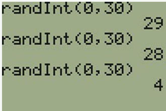
Figure 1.2.10 — TI calculator screen showing the randInt command used to generate sample IDs.

Besides simple random sampling, several other methods also use a chance process. The best-known are the stratified sample, the cluster sample, and the systematic sample.

Definition 1.2.6: Stratified Sample

To choose a stratified sample, divide the population into groups called strata and then take a proportionate random sample from each stratum.

For example, you could stratify your college population by department, then take a proportionate simple random sample from each department. Number each member of the first department and use simple random sampling to pick a proportionate number; repeat for every department. All the names picked across all departments make up the stratified sample.

Definition 1.2.7: Cluster Sample

To choose a cluster sample, divide the population into clusters (groups), randomly select some of the clusters, and include every member of the chosen clusters.

For example, divide your college faculty by department — the departments are the clusters. Number the departments, use simple random sampling to choose four of them, and every faculty member in those four departments is in the cluster sample.

Definition 1.2.8: Systematic Sample

To choose a systematic sample, randomly select a starting point and then take every \(k\)-th piece of data from a list of the population.

For example, suppose you must do a phone survey from a phone book with 20,000 residential listings, and you need 400 names. Number the population 1 through 20,000, use a simple random sample to pick the first name, then take every fiftieth name after that until you have 400 (wrapping back to the start of the list if needed). Systematic sampling is popular because it is so simple.

Definition 1.2.9: Convenience Sample

A convenience sample is a non-random sample that uses whatever results are readily available.

Sampling carelessly can wreck a study before a single number is crunched. Mailed surveys that people return on their own are notoriously biased, because the people who bother to reply are rarely a fair cross-section of everyone. Whenever possible, the person running the survey should choose the respondents rather than letting respondents choose themselves. Keep this in mind as we sort the next batch of scenarios — the trap in each one is almost always who got left out.

For example, a software store runs a marketing study by interviewing whoever happens to be browsing in the store that day. Convenience sampling can give very good results in some cases and highly biased results (results that favor certain outcomes) in others.

There is also a subtle choice about whether a chosen member can be picked again. Sampling with replacement is truly random: once a member is picked, they go back into the population and could be chosen more than once. For practical reasons, though, most real surveys use sampling without replacement — a member can be chosen only once. When samples are small compared with a large population, sampling without replacement is approximately the same as sampling with replacement, because the chance of drawing the same person twice is tiny. The distinction only becomes a real mathematical issue when the population is small.

When you analyze data, watch for two kinds of error. A sampling error is caused by the sampling process itself — for example, the sample may not be large enough. A nonsampling error comes from factors unrelated to sampling — for example, a defective counting device. A sample will never be exactly representative of its population, so some sampling error is always present; as a rule, the larger the sample, the smaller the sampling error.

Finally, a sampling bias occurs when some members of the population are less likely to be chosen than others (remember, every member should have an equally likely chance). When bias creeps in, the conclusions drawn about the population can be flat wrong.

Gathering information about an entire population usually costs too much or is simply impossible. Instead, we study a sample of the population. A good sample has the same characteristics as the population it represents, and statisticians use various methods of random sampling to try to achieve that. In every form of random sampling, each member of the population starts out with an equal chance of being selected. Each method has its own pros and cons.

1.2.4 Evaluating Studies Critically

We should read statistical studies critically and analyze them before accepting their results. Watch for these common problems:

Problems with the Sample

A sample must be representative of the population. A sample that is not representative is biased, and biased samples give results that are inaccurate and not valid.

Self-Selected Samples

Responses only from people who choose to respond — such as call-in surveys — are often unreliable.

Sample-Size Issues

Samples that are too small may be unreliable; larger samples are better when possible. Sometimes small samples are unavoidable and still useful — for example, crash-testing cars or medical testing for rare conditions.

Undue Influence

Collecting data or asking questions in a way that influences the response.

Non-Response or Refusal to Participate

When many subjects do not respond, the collected responses may no longer represent the population. People with strong positive or negative opinions are often the ones who answer, which skews the results.

Causality

A relationship between two variables does not mean one causes the other. They may be related (correlated) only because of a third, lurking variable.

Self-Funded or Self-Interest Studies

A study run by a person or organization to support their own claim. Ask whether it is impartial. Do not automatically assume it is bad — or good — but evaluate it on the merits of the work done.

Misleading Use of Data

Improperly displayed graphs, incomplete data, or missing context.

Confounding

When the effects of several factors on a response cannot be separated, the factors are confounded, and it becomes difficult or impossible to draw valid conclusions about any single factor.

A magnifying glass over a survey form, signaling the need to evaluate studies critically.

As a class, decide whether each of the following samples is representative. If it is not, discuss why.

1. To find the average GPA of all students at a university, use all honor students as the sample.

2. To find the most popular cereal among children under ten, stand outside a large supermarket for three hours and speak to every twentieth child under ten who enters.

3. To find the average annual income of all U.S. adults, sample U.S. Representatives: treat each state as a stratum, use simple random sampling to select states, then survey every Representative in the chosen states.

4. To find the proportion of people who take public transportation to work, sit on a bench in Central Park and interview the next 20 people who sit beside you.

5. To find the average cost of a two-day hospital stay in Massachusetts, survey 100 hospitals across the state using simple random sampling.

Before we move on to the worked examples that drill these sampling types, it helps to name the move you will make each time. For every scenario, ask two questions in order: Was chance used at all? If not, it is convenience sampling. If chance was used, what got divided and what got selected? If you split the population into groups and sampled within every group, it is stratified; if you picked a few whole groups and took everyone inside them, it is cluster; if you walked down a list grabbing every \(k\)-th name, it is systematic; and if every individual had an equal, independent shot, it is simple random. The next two examples are pure practice at running that checklist quickly.

Students walking on a college campus, the setting for the tuition sampling example.

A youth soccer team, the scenario behind the stratified sampling example.

1.2.5 Variation in Data and Samples

If we examined two samples from the same population — even using random sampling for both — they would not come out exactly the same. Just as there is variation in data, there is variation in samples. As you get used to sampling, this variability will start to feel natural.

In the Confidence Intervals chapter, you will meet sample-size formulas that tell you how big a sample to take. The required size depends on the precision you want, not on the size of the population. It can feel counterintuitive, but a sample of 1,000 can adequately represent a population of 100,000 or even 1,000,000, as long as you want the same level of precision. When you reach those formulas, notice that population size never appears in them.

Variation in Data

Variation is present in any set of data. For example, 16-ounce cans of a beverage may hold a little more or a little less than 16 ounces. In one study, eight 16-ounce cans were measured and produced these amounts (in ounces):

15.8; 16.1; 15.2; 14.8; 15.8; 15.9; 16.0; 15.5

The measured amounts vary because different people make the measurements, or because exactly 16 ounces was never put in the cans in the first place. Manufacturers regularly run tests to check whether the amount in a 16-ounce can falls within the desired range.

Be aware that your data may differ a bit from data someone else collects for the same purpose — that is completely natural. But if two people collecting the same data get very different results, it is time to reevaluate the data-taking methods and accuracy.

Variation in Samples

As noted, two or more random samples from the same population will likely differ from each other. Suppose Doreen and Jung both study the average nightly sleep of students at their college, each taking samples of 500 students. Doreen uses systematic sampling and Jung uses cluster sampling, so their samples will differ. Even if they used the same method, their samples would almost certainly still differ — and neither would be wrong.

Think about what makes Doreen's and Jung's samples different. If they took larger samples, their results (the average sleep time) might land closer to the true population average — but the two samples would still, in all likelihood, differ from each other. This variability in samples cannot be stressed enough.

1.2.6 Size of a Sample

The size of a sample (often called the number of observations) matters. The examples in this book so far have been small. Samples of a few hundred observations — or even fewer — are enough for many purposes. In polling, samples of about 1,200 to 1,500 observations are considered large and good enough, if the survey is random and well done. You will learn why when you study confidence intervals.

Be aware that many large samples are still biased. Call-in surveys, for example, are invariably biased because people choose whether or not to respond.

A crowd of people, illustrating how sample size relates to representing a large population.

Divide into groups of two, three, or four. Your instructor will give each group one six-sided die. Try this experiment twice: roll one fair die 20 times and record how many ones, twos, threes, fours, fives, and sixes you get in Table 1.2.6 and Table 1.2.7 ("frequency" is the number of times a particular face appears).

Table 1.2.6 — First experiment (20 rolls).
Face on DieFrequency
1
2
3
4
5
6
Table 1.2.7 — Second experiment (20 rolls).
Face on DieFrequency
1
2
3
4
5
6

Did the two experiments give the same results? Probably not. If you ran the experiment a third time, would you expect results identical to the first or second? Why or why not? Which experiment had the "correct" results? They both did — the job of the statistician is to see through the variability and draw appropriate conclusions.

Appendix — Additional Examples and Practice

The following items were carried over from a second source text covering the same material. They are kept here as additional practice rather than folded into the main flow.

Example 1.A1

Is \(\mu\) a parameter or a statistic? What about \(\hat{p}\)?

Solution

\(\mu\) is a parameter because it refers to the average of the entire population. \(\hat{p}\) is a statistic because it is calculated from a sample.

Example 1.A2

A systematic sample is not the same as a simple random sample. Give an example of a sample that can come from a simple random sample but not from a systematic random sample.

Solution

Answers can vary. If we take a sample of size 3, it is possible to select players numbered 1, 2, and 3 in a simple random sample. Such a sample would be impossible from a systematic sample, because systematic sampling spaces selections evenly across the list. The "every group of the same size is equally likely" property of simple random samples does not hold for other types of random samples.

Figure 1.2.11 — Two panels comparing sampling methods: (top) simple random sampling selects 18 cases at random; (bottom) systematic random sampling selects every 7th individual.

Sometimes a variable is known to be associated with the quantity we want to estimate. In that case a stratified random sample may be best. Stratified sampling is a divide-and-conquer strategy: the population is split into strata so that similar cases are grouped together, and a sampling method (usually simple random sampling) selects a certain number or proportion within each stratum. In a baseball-salary example, the 30 teams could be the strata — some teams have far more money than others.

Try It Now 1.2.14

How and why should randomization be incorporated into a matched pairs design?

Solution

Randomization should decide, within each matched pair, which member receives which treatment. This guards against hidden bias: if the experimenter always assigned the treatment to (say) the first member of every pair, any difference between "first" and "second" members would get confounded with the treatment effect. Randomizing the assignment within each pair ensures that lurking differences are, on average, balanced across the two treatment groups, so the observed difference can be attributed to the treatment rather than to how subjects were ordered.

Illustration of a matched-pairs experimental design.

Example 1.A3

This example examines the relationship between a county's population change from 2010 to 2017 and its median household income, shown as a scatterplot. Are these variables associated?

Solution

The larger the median household income for a county, the higher its observed population growth. The trend is not true for every single county, but it is clearly visible in the plot. Because there is some relationship between the variables, they are associated — here, positively associated, since higher income tends to come with higher population growth. (By contrast, when counties with more units in multi-unit structures tend to have lower homeownership, those variables are negatively associated.)

If two variables show no evident relationship, they are independent.

Association Does Not Imply Causation

Labeling variables as explanatory and response does not guarantee the relationship is actually causal, even when an association is identified. We use these labels only to track which variable we suspect affects the other.

In many cases the relationship is complex or unknown. It may be unclear whether variable \(A\) explains variable \(B\) or vice versa. For example, a protein called REST is much depleted in people with Alzheimer's disease. This raises hopes for a treatment, but it is still unknown whether the lack of the protein causes brain deterioration, whether brain deterioration causes the depletion, or whether some third variable causes both. We simply do not know whether the lack of the protein is an explanatory variable or a response variable — perhaps it is both.

Example 1.A4

For the baseball example, briefly explain how to select a stratified random sample of size \(n = 120\).

Solution

Let each team serve as a stratum. Take a simple random sample of 4 players from each of the 30 teams, yielding \(4 \times 30 = 120\) players. Stratified sampling differs from simple random sampling: this approach makes it impossible for an entire single team (say, the Yankees) to be selected as the whole sample.

Association ≠ Causation

In general, association does not imply causation, and causation can only be inferred from a randomized experiment.

Try It Now 1.2.15

We can easily access ratings for products, sellers, and companies online. These ratings come only from people who go out of their way to provide one. If 50% of online reviews for a product are negative, does this mean that 50% of buyers are dissatisfied?

Solution

No. Reviewers are self-selected — people with strong opinions (especially negative ones) are far more likely to bother writing a review than satisfied customers who quietly move on. So the 50% figure describes the reviewers, not all buyers. The reviews are a biased, non-representative sample of the buyer population.

Watch Out For Bias

Undercoverage bias, non-response bias, and response bias can all exist within a random sample. Always determine how a sample was chosen, ask what proportion of people failed to respond, and critically examine the wording of the questions.

When there is no bias, increasing the sample size tends to increase the precision and reliability of the estimate. When a sample is biased, it may be impossible to extract helpful information from the data, even if the sample is very large.

Try It Now 1.2.16

A researcher mails questionnaires to 50 randomly selected households asking whether they support adding a traffic light in their neighborhood. Only 20% of the questionnaires are returned, so she mails questionnaires to 50 more randomly selected households in the same neighborhood. Comment on the usefulness of this approach.

Solution

Mailing more questionnaires does not fix the core problem: non-response bias. The 20% who returned the first round are likely the people with the strongest opinions (for or against the traffic light), so their responses may not represent the neighborhood. Sending 50 more questionnaires will probably yield the same low return rate and the same self-selected, opinionated respondents. To improve usefulness, she should focus on raising the response rate — follow-up reminders, in-person or phone contact — rather than simply mailing out more surveys.

Problem Set 1.2

For problems 17 through 21, use the following information.

A study was done to determine the age, number of times per week, and the duration (amount of time) of residents using a local park in San Antonio, Texas. The first house in the neighborhood around the park was selected randomly, and then the resident of every eighth house in the neighborhood around the park was interviewed.

Problem 17. "Number of times per week" is what type of data?

a) qualitative (categorical)

b) quantitative discrete

c) quantitative continuous

Solution

Step 1 — Classify the variable: "Number of times per week" is a count, so it is quantitative (numeric), not categorical.

Step 2 — Discrete or continuous? A count can only take whole-number values (0, 1, 2, …); you cannot use the park 2.5 times in a counting sense, so it is discrete.

Answer: b) quantitative discrete.

Problem 18. The sampling method was

a) simple random

b) systematic

c) stratified

d) cluster

Solution

Step 1 — Identify the selection rule: Starting from one randomly chosen first house, the interviewer then takes every eighth house — a fixed interval down the list.

Step 2 — Match to a sampling method: Choosing every \(k\)th element from an ordered list (here \(k = 8\)) is the definition of systematic sampling.

Answer: b) systematic.

Problem 19. "Duration (amount of time)" is what type of data?

a) qualitative (categorical)

b) quantitative discrete

c) quantitative continuous

Solution

Step 1 — Classify the variable: "Duration (amount of time)" is measured numerically, so it is quantitative.

Step 2 — Discrete or continuous? Time can take any value in a range (e.g., 12.4 minutes, 12.43 minutes); measurements are not restricted to whole numbers, so it is continuous.

Answer: c) quantitative continuous.

Problem 20. The colors of the houses around the park are what kind of data?

a) qualitative (categorical)

b) quantitative discrete

c) quantitative continuous

Solution

Step 1 — Classify the variable: A house color (red, blue, white, …) is a label/category, not a number.

Step 2 — Confirm the type: Since the values are names rather than measurements or counts, the data are qualitative.

Answer: a) qualitative (categorical).

Problem 21. The population is ____________.

Solution

Step 1 — Recall the definition: The population is every individual the study aims to describe.

Step 2 — Apply it to the park study: The researchers want to characterize the people who use this San Antonio park, so the population is all of those users.

Answer: The population is all the people (residents) who use that local park in San Antonio.

For problems 6 through 9, determine the type of sampling used (simple random, stratified, systematic, cluster, or convenience).

Problem 22. A group of test subjects is divided into twelve groups; then four of the groups are chosen at random.

Solution

Step 1 — Identify the selection rule: Twelve groups are formed, then 4 entire groups are chosen at random and everyone in those groups is used.

Step 2 — Match to a sampling method: Sampling whole pre-existing groups (clusters) rather than individuals is cluster sampling.

Answer: Cluster sampling.

Problem 23. A market researcher polls every tenth person who walks into a store.

Solution

Step 1 — Identify the selection rule: The researcher polls every tenth person entering the store — a fixed interval applied to an ordered stream of people.

Step 2 — Match to a sampling method: Selecting every \(k\)th element (\(k = 10\)) is systematic sampling.

Answer: Systematic sampling.

Problem 24. The first 50 people who walk into a sporting event are polled on their television preferences.

Solution

Step 1 — Identify the selection rule: The first 50 people through the door are polled simply because they are easiest to reach.

Step 2 — Match to a sampling method: Choosing whoever is most readily available, with no random mechanism, is convenience sampling.

Answer: Convenience sampling.

Problem 25. A computer generates 100 random numbers, and 100 people whose names correspond with the numbers on the list are chosen.

Solution

Step 1 — Identify the selection rule: A computer produces 100 random numbers, and the 100 people matching those numbers are selected; every person on the list has an equal chance.

Step 2 — Match to a sampling method: Equal-probability selection of individuals by a random device is simple random sampling.

Answer: Simple random sampling.

For problems 10 through 17, use the following Researcher A and Researcher B respiratory-virus data sets (40 patients each).

Studies are often done by pharmaceutical companies to determine the effectiveness of a treatment program. Suppose that a new drug is currently under study to address a respiratory virus. It is given to patients once the patient exhibits symptoms of the virus. Of interest is the average (mean) length of time in days from the time the patient starts the treatment until the symptoms are alleviated. Two researchers each follow a different set of 40 patients with the respiratory virus from the start of treatment until the symptoms are alleviated. The following data (in days) are collected.

Researcher A: 3; 4; 11; 15; 16; 17; 22; 44; 37; 16; 14; 24; 25; 15; 26; 27; 33; 29; 35; 44; 13; 21; 22; 10; 12; 8; 40; 32; 26; 27; 31; 34; 29; 17; 8; 24; 18; 47; 33; 34

Researcher B: 3; 14; 11; 5; 16; 17; 28; 41; 31; 18; 14; 14; 26; 25; 21; 22; 31; 2; 35; 44; 23; 21; 21; 16; 12; 18; 41; 22; 16; 25; 33; 34; 29; 13; 18; 24; 23; 42; 33; 29

Problem 26. Complete the tables using the data provided.

Table 1.2.8 — Researcher A survival-length frequency table (to complete).
Survival Length (in days)FrequencyRelative FrequencyCumulative Relative Frequency
0.5–6.5
6.5–12.5
12.5–18.5
18.5–24.5
24.5–30.5
30.5–36.5
36.5–42.5
42.5–48.5
Table 1.2.9 — Researcher B survival-length frequency table (to complete).
Survival Length (in days)FrequencyRelative FrequencyCumulative Relative Frequency
0.5–6.5
6.5–12.5
12.5–18.5
18.5–24.5
24.5–30.5
30.5–36.5
36.5–45.5
Solution

Step 1 — Set up the bins: Each row counts how many of the \(n = 40\) survival times fall in that interval (lower bound exclusive, upper bound inclusive). Relative frequency \(= \dfrac{\text{frequency}}{40}\), and cumulative relative frequency is the running total of relative frequencies.

Step 2 — Tally Researcher A (Table 1.2.8): Counting Researcher A's 40 values into each bin gives frequencies \(2, 5, 9, 5, 7, 7, 2, 3\) (sum \(= 40\)).

Survival Length Frequency Rel. Freq. Cum. Rel. Freq.
0.5–6.5 2 0.050 0.050
6.5–12.5 5 0.125 0.175
12.5–18.5 9 0.225 0.400
18.5–24.5 5 0.125 0.525
24.5–30.5 7 0.175 0.700
30.5–36.5 7 0.175 0.875
36.5–42.5 2 0.050 0.925
42.5–48.5 3 0.075 1.000

Step 3 — Tally Researcher B (Table 1.2.9): Counting Researcher B's 40 values gives frequencies \(3, 2, 11, 8, 6, 6, 4\) (sum \(= 40\)).

Survival Length Frequency Rel. Freq. Cum. Rel. Freq.
0.5–6.5 3 0.075 0.075
6.5–12.5 2 0.050 0.125
12.5–18.5 11 0.275 0.400
18.5–24.5 8 0.200 0.600
24.5–30.5 6 0.150 0.750
30.5–36.5 6 0.150 0.900
36.5–45.5 4 0.100 1.000

Step 4 — Check: Each frequency column sums to 40 and each final cumulative relative frequency equals 1.000, confirming the tables are complete.

Answer: The completed Researcher A and Researcher B frequency tables are shown above; frequencies are \(2,5,9,5,7,7,2,3\) for A and \(3,2,11,8,6,6,4\) for B, both summing to 40 with cumulative relative frequency reaching 1.000.

Problem 27. Determine what the key term data refers to in the above example for Researcher A.

Solution

Step 1 — Recall the definition: Data are the actual recorded values of the variable for the members of the sample.

Step 2 — Apply it to Researcher A: For Researcher A, the data are the 40 measured survival lengths (3, 4, 11, 15, … , 34 days).

Answer: The data are the set of 40 recorded survival times (in days) for Researcher A's patients.

Problem 28. List two reasons why the data may differ.

Solution

Step 1 — Think about the source of variation: The two researchers followed different sets of 40 patients, and individual patients respond differently to the drug.

Step 2 — List two reasons: (1) The two samples consist of different individuals, so natural patient-to-patient variation produces different values; (2) differences in conditions or methodology — for example, how the patients were selected, regional or demographic differences, severity of illness at start, or measurement/recording differences — can shift the results.

Answer: The data may differ because (1) each researcher sampled a different group of patients (sampling variability), and (2) factors such as how patients were chosen, their differing health conditions/severity, or measurement differences vary between the two studies.

Problem 29. Can you tell if one researcher is correct and the other one is incorrect? Why?

Solution

Step 1 — Interpret "correct": Each researcher honestly recorded the survival times for their own randomly chosen sample.

Step 2 — Explain why neither is wrong: Two different random samples from the same population are expected to give different results; that difference is sampling variability, not error. Neither set of data is "correct" or "incorrect" — both are valid samples.

Answer: No. Both researchers can be reporting accurate data; the differences simply reflect natural sampling variability between two different groups of patients, so one cannot be declared right and the other wrong.

Problem 30. Would you expect the data to be identical? Why or why not?

Solution

Step 1 — Consider what identical data would require: Identical data would mean both researchers happened to draw the same 40 individuals (or the same exact values), which is essentially impossible for two separate random samples.

Step 2 — Explain: Because the samples contain different patients and patients vary in how they respond, the recorded values will differ.

Answer: No, we would not expect the data to be identical. The two researchers sampled different patients, and individual responses vary, so the two data sets will naturally differ even though they describe the same population.

Problem 31. Suggest at least two methods the researchers might use to gather random data.

Solution

Step 1 — Recall what "random" requires: A random method gives every patient a known, fair chance of being selected, removing the researcher's personal choice.

Step 2 — Suggest two methods: (1) Simple random sampling — assign every eligible patient a number and use a random number generator or table to pick 40; (2) systematic sampling — order all eligible patients and select every \(k\)th one starting from a random start. (Stratified or cluster random sampling are also acceptable.)

Answer: Two workable methods are simple random sampling (number every patient and draw 40 with a random number generator) and systematic sampling (pick every \(k\)th patient from an ordered list after a random start).

Problem 32. Suppose that the first researcher conducted his survey by randomly choosing one state in the nation and then randomly picking 40 patients from that state. What sampling method would that researcher have used?

Solution

Step 1 — Identify the two stages: First a state is chosen at random; then 40 patients are chosen at random from within that one state.

Step 2 — Match to a sampling method: Selecting whole geographic group(s) at random and then sampling within them is cluster sampling (the state is the cluster).

Answer: Cluster sampling.

Problem 33. Suppose that the second researcher conducted his survey by choosing 40 patients he knew. What sampling method would that researcher have used? What concerns would you have about this data set, based upon the data collection method?

Solution

Step 1 — Identify the selection rule: The researcher used 40 patients he already knew, choosing them because they were easy to access rather than by any random mechanism.

Step 2 — Match to a sampling method: Selecting readily available, familiar subjects is convenience sampling.

Step 3 — State the concern: A convenience sample is likely biased and not representative of the whole population — patients the researcher knows may share characteristics (location, health habits, demographics) that differ from typical patients, so conclusions drawn from this sample may not generalize.

Answer: Convenience sampling. The main concern is bias: because the patients were not chosen randomly but because the researcher knew them, the sample may not represent the broader population, making the results unreliable for general conclusions.

For problems 18 through 22, two researchers are gathering data on hours of video games played by school-aged children and young adults. They each randomly sample different groups of 150 students from the same school. They collect the following data.

Table 1.2.10 — Researcher A: hours of video games played per week.
Hours Played per WeekFrequencyRelative FrequencyCumulative Relative Frequency
0–2260.170.17
2–4300.200.37
4–6490.330.70
6–8250.170.87
8–10120.080.95
10–1280.051
Table 1.2.11 — Researcher B: hours of video games played per week.
Hours Played per WeekFrequencyRelative FrequencyCumulative Relative Frequency
0–2480.320.32
2–4510.340.66
4–6240.160.82
6–8120.080.90
8–10110.070.97
10–1240.03

Problem 34. Give a reason why the data may differ.

Solution

Step 1 — Recognize the source of variability: Two researchers each surveyed a different set of respondents, so the two data sets are independent samples drawn from the population. Random sampling means no two samples will be identical.

Step 2 — Identify a concrete reason: Differences arise from sampling variability — each sample contains different individuals whose video-game habits differ. Other contributing factors include how the question was worded, when and where each survey was administered, and ordinary measurement/reporting error.

Answer: The data differ because each researcher surveyed a different random sample of people; sampling variability (plus possible differences in question wording, timing, and respondent honesty) produces different results even when both studies are run correctly.

Problem 35. Would the sample size be large enough if the population is the students in the school?

Solution

Step 1 — Compare sample size to population size: "The students in the school" is a relatively small, well-defined population. A survey covering a sizeable fraction of that population gives a representative picture.

Step 2 — Judge adequacy: Because the population is limited to one school, even a few hundred respondents would represent a large share of the whole, so the sample is large enough to draw reliable conclusions about that school.

Answer: Yes. For a population as small and specific as the students in one school, the sample is large enough to be reliable.

Problem 36. Would the sample size be large enough if the population is school-aged children and young adults in the United States?

Solution

Step 1 — Reconsider the population size: "School-aged children and young adults in the United States" is an enormous and highly diverse population numbering in the tens of millions.

Step 2 — Judge adequacy: A sample taken at a single school cannot capture the geographic, economic, and cultural diversity of the whole country, and it is a tiny fraction of that population, so it is neither large enough nor representative.

Answer: No. The sample is far too small and not representative enough to support conclusions about all school-aged children and young adults in the United States.

Problem 37. Researcher A concludes that most students play video games between four and six hours each week. Researcher B concludes that most students play video games between two and four hours each week. Who is correct?

Solution

Step 1 — Examine what each researcher is claiming: Each conclusion describes the typical play time for that researcher's own sample. The two samples are different sets of people.

Step 2 — Decide whether one must be wrong: Because the two samples differ, both conclusions can be valid descriptions of their respective samples. Neither is necessarily "correct" for the whole population — the difference reflects sampling variability, not error.

Answer: Neither is provably correct. Each conclusion accurately describes that researcher's own sample; the discrepancy is due to sampling variability, so we cannot say one researcher is right and the other wrong.

Problem 38. As part of a way to reward students for participating in the survey, the researchers gave each student a gift card to a video game store. Would this affect the data if students knew about the award before the study?

Solution

Step 1 — Consider how an incentive changes behavior: If students knew about the gift card in advance, the reward could influence who chose to participate and how they responded.

Step 2 — Identify the bias: Advance knowledge of a prize attracts self-selected participants (people interested in video games / gift cards) and may encourage rushed or exaggerated answers, biasing the data.

Answer: Yes. Knowing about the reward beforehand could bias the data through self-selection and influenced responses; a reward given only after participation, with no prior knowledge, would be far less likely to affect the results.

For problems 23 through 27, a pair of studies was performed to measure the effectiveness of a new software program designed to help stroke patients regain their problem-solving skills. Patients were asked to use the software program twice a day, once in the morning and once in the evening. The studies observed 200 stroke patients recovering over a period of several weeks. The first study collected the data in Table 1.2.12. The second study collected the data in Table 1.2.13.

Table 1.2.12 — First study of the stroke-recovery software.
GroupShowed improvementNo improvementDeterioration
Used program1424315
Did not use program7211018
Table 1.2.13 — Second study of the stroke-recovery software.
GroupShowed improvementNo improvementDeterioration
Used program1057419
Did not use program89994

Problem 39. Given what you know, which study is correct?

Solution

Step 1 — Recall that independent samples can differ: The two studies followed different groups of 200 stroke patients, so different counts are expected from sampling variability alone.

Step 2 — Decide whether one is "correct": Neither study is inherently right or wrong. Both are legitimate observations of different samples; without more information we cannot label one correct.

Answer: Neither can be declared correct. Both are valid studies of different patient groups, and the differing results reflect sampling variability rather than one study being wrong.

Problem 40. The first study was performed by the company that designed the software program. The second study was performed by the American Medical Association. Which study is more reliable?

Solution

Step 1 — Look for a conflict of interest: The first study was run by the company that makes the software, giving it a financial stake in a favorable result. The second was run by the American Medical Association, an independent professional body.

Step 2 — Judge reliability: An independent organization with no financial interest in the outcome is less prone to bias, so its findings carry more credibility.

Answer: The second study (American Medical Association) is more reliable, because it was conducted by an independent party without a financial stake in the result, whereas the company-run study has a conflict of interest.

Problem 41. Both groups that performed the study concluded that the software works. Is this accurate?

Solution

Step 1 — Compare the two data sets: In the first study, 142 of 200 program users improved (71%) versus 72 of 200 non-users (36%). In the second study, 105 of 200 users improved (52.5%) versus 89 of 200 non-users (44.5%).

Step 2 — Assess the shared conclusion: Both studies show users improving at a higher rate than non-users, so the qualitative claim "the software is associated with improvement" is consistent across both, even though the size of the effect differs.

Answer: It is accurate to say both studies found a higher improvement rate among software users than non-users. However, the second (independent) study shows a much smaller advantage, so the strength of the effect is uncertain — the direction of the conclusion is consistent, but the magnitude is not.

Problem 42. The company takes the two studies as proof that their software causes mental improvement in stroke patients. Is this a fair statement?

Solution

Step 1 — Separate association from causation: The studies are observational: patients were grouped by whether they used the software, not randomly assigned. Observed improvement could stem from confounding factors rather than the software itself.

Step 2 — Apply the causation rule: A correlation between software use and improvement does not by itself prove the software causes improvement. Only a properly controlled, randomized experiment can establish causation.

Answer: No. The studies are observational and show only an association, not causation. Without a randomized controlled experiment, the company cannot fairly claim the software causes mental improvement.

Problem 43. Patients who used the software were also a part of an exercise program whereas patients who did not use the software were not. Does this change the validity of the conclusions from Problem 41?

Solution

Step 1 — Identify the new confounding variable: Program users were also in an exercise program while non-users were not. Exercise itself can aid stroke recovery, so it is confounded with software use.

Step 2 — Reassess the conclusion from 1.2.25: Because the two groups differ in more than just software use, any improvement could be due to the exercise rather than the software. The groups are no longer comparable.

Answer: Yes, it changes the validity. Exercise is a confounding variable that differs between the groups, so the observed improvement cannot be attributed to the software alone; the conclusions from Problem 41 are weakened.

Problem 44. Is a sample size of 1,000 a reliable measure for a population of 5,000?

Solution

Step 1 — Compute the sampling fraction: The sample is \(1{,}000\) out of a population of \(5{,}000\): $$\frac{1{,}000}{5{,}000} = 0.20 = 20%.$$

Step 2 — Judge reliability: A randomly chosen sample of 1,000 is a large absolute size and covers 20% of the population, which is more than adequate to estimate population characteristics reliably (provided it is randomly selected).

Answer: Yes. A sample of 1,000 (20% of the population of 5,000), if randomly selected, is large enough to be a reliable measure.

Problem 45. Is a sample of 500 volunteers a reliable measure for a population of 2,500?

Solution

Step 1 — Compute the sampling fraction: The sample is \(500\) out of a population of \(2{,}500\): $$\frac{500}{2{,}500} = 0.20 = 20%.$$

Step 2 — Account for self-selection: Twenty percent is a substantial fraction, but these are volunteers. Volunteer (self-selected) samples are prone to bias because volunteers may differ systematically from the general population.

Answer: The size (500, or 20% of 2,500) is adequate, but because the participants are self-selected volunteers, the sample may be biased and is therefore not necessarily reliable. A randomly selected sample of the same size would be preferable.

Problem 46. A question on a survey reads: "Do you prefer the delicious taste of Brand X or the taste of Brand Y?" Is this a fair question?

Solution

Step 1 — Read the wording critically: The question describes Brand X as having a "delicious taste" while describing Brand Y's taste neutrally. The adjective primes the respondent toward Brand X.

Step 2 — Identify the flaw: This is a leading question — its phrasing biases the answer rather than letting the respondent choose freely.

Answer: No, it is not a fair question. The word "delicious" applied only to Brand X makes it a leading (biased) question; a fair version would describe both brands neutrally, e.g., "Do you prefer the taste of Brand X or the taste of Brand Y?"

Problem 47. Is a sample size of two representative of a population of five?

Solution

Step 1 — Compute the sampling fraction: A sample of \(2\) from a population of \(5\): $$\frac{2}{5} = 0.40 = 40%.$$

Step 2 — Judge representativeness: Although 40% is a large fraction, the absolute sample size of two is far too small to capture the variation in the population; just one unusual individual would dominate the result.

Answer: No. A sample of size two is too small to be representative of a population of five, despite being 40% of it — there is not enough data to reflect the population's variability.

Problem 48. Is it possible for two experiments to be well run with similar sample sizes to get different data?

Solution

Step 1 — Recall the role of randomness: Even with careful design and equal sample sizes, two experiments draw different random samples from the population.

Step 2 — Conclude: Random sampling guarantees that two independent, well-run experiments will almost always produce somewhat different data. This is expected sampling variability, not a sign of error.

Answer: Yes. Two well-run experiments with similar sample sizes can easily produce different data because they sample different individuals; this is normal sampling variability.

For problems 33 through 42, identify the type of data that would be used to describe a response (quantitative discrete, quantitative continuous, or qualitative), and give an example of the data.

Problem 49. number of tickets sold to a concert

Solution

Step 1 — Decide qualitative vs. quantitative: Number of tickets sold is a count, so it is numerical — quantitative.

Step 2 — Decide discrete vs. continuous: Counts take only whole-number values (you cannot sell 412.5 tickets), so the data are quantitative discrete.

Answer: Quantitative discrete. Example: 412 tickets sold to a particular concert.

Problem 50. percent of body fat

Solution

Step 1 — Decide qualitative vs. quantitative: Percent of body fat is a measured numerical quantity, so it is quantitative.

Step 2 — Decide discrete vs. continuous: It is measured on a scale and can take any value in a range (including fractions), so the data are quantitative continuous.

Answer: Quantitative continuous. Example: a body-fat measurement of 18.6%.

Problem 51. favorite baseball team

Solution

Step 1 — Decide qualitative vs. quantitative: A favorite baseball team is a name or category, not a number, so it is qualitative (categorical).

Step 2 — Confirm: There is no meaningful arithmetic on team names, which confirms the data are qualitative.

Answer: Qualitative. Example: the San Francisco Giants.

Problem 52. time in line to buy groceries

Solution

Step 1 — Decide qualitative vs. quantitative: Time waiting in line is a measured numerical quantity, so it is quantitative.

Step 2 — Decide discrete vs. continuous: Time can take any value in a range (e.g., 4.3 minutes), so the data are quantitative continuous.

Answer: Quantitative continuous. Example: 4.3 minutes spent in line.

Problem 53. number of students enrolled at Evergreen Valley College

Solution

Step 1 — Decide qualitative vs. quantitative: Number of students enrolled is a count, so it is numerical — quantitative.

Step 2 — Decide discrete vs. continuous: Counts are whole numbers (you cannot enroll a fraction of a student), so the data are quantitative discrete.

Answer: Quantitative discrete. Example: 9,800 students enrolled.

Problem 54. most-watched television show

Solution

Step 1 — Decide qualitative vs. quantitative: A most-watched television show is a title/category, not a number, so it is qualitative (categorical).

Step 2 — Confirm: Show titles cannot be averaged or otherwise computed with, confirming the data are qualitative.

Answer: Qualitative. Example: the most-watched show being Jeopardy!

Problem 55. brand of toothpaste

Solution

Step 1 — Decide qualitative vs. quantitative: A brand of toothpaste is a name or category, not a number, so it is qualitative (categorical).

Step 2 — Confirm: Brand names support no arithmetic, confirming the data are qualitative.

Answer: Qualitative. Example: the brand Colgate.

Problem 56. distance to the closest movie theatre

Solution

Step 1 — Decide qualitative vs. quantitative: Distance is a measured numerical quantity, so it is quantitative.

Step 2 — Decide discrete vs. continuous: Distance can take any value in a range (e.g., 2.7 miles), so the data are quantitative continuous.

Answer: Quantitative continuous. Example: 2.7 miles to the closest movie theatre.

Problem 57. age of executives in Fortune 500 companies

Solution

Step 1 — Decide qualitative vs. quantitative: Age is a measured numerical quantity, so it is quantitative.

Step 2 — Decide discrete vs. continuous: Age is measured on a continuous scale (it can take any value, e.g., 52.4 years), so the data are quantitative continuous.

Answer: Quantitative continuous. Example: an executive aged 52.4 years.

Problem 58. number of competing computer spreadsheet software packages

Solution

Step 1 — Decide qualitative vs. quantitative: Number of competing software packages is a count, so it is numerical — quantitative.

Step 2 — Decide discrete vs. continuous: Counts take only whole-number values, so the data are quantitative discrete.

Answer: Quantitative discrete. Example: 5 competing spreadsheet packages.

For problems 43 and 44, a study was done to determine the age, number of times per week, and the duration (amount of time) of resident use of a local park in San Jose. The first house in the neighborhood around the park was selected randomly and then every 8th house in the neighborhood around the park was interviewed.

Problem 59. "Number of times per week" is what type of data?

a) qualitative

b) quantitative discrete

c) quantitative continuous

Solution

Step 1 — Classify the variable: "Number of times per week" a resident uses the park is a count of visits.

Step 2 — Decide the data type: A count takes only whole-number values, so it is numerical and discrete — quantitative discrete. It is not qualitative (it is a number) and not continuous (you cannot use the park 3.5 times in the counting sense).

Answer: b) quantitative discrete.

Problem 60. "Duration (amount of time)" is what type of data?

a) qualitative

b) quantitative discrete

c) quantitative continuous

Solution

Step 1 — Classify the variable: "Duration (amount of time)" measures how long each resident uses the park.

Step 2 — Decide the data type: Time is measured on a continuous scale and can take any value in a range (e.g., 1.75 hours), so it is quantitative continuous. It is not qualitative (it is a number) and not discrete (it is not a whole-number count).

Answer: c) quantitative continuous.

Problem 61. Airline companies are interested in the consistency of the number of babies on each flight, so that they have adequate safety equipment. Suppose an airline conducts a survey. Over Thanksgiving weekend, it surveys six flights from Boston to Salt Lake City to determine the number of babies on the flights. It determines the amount of safety equipment needed by the result of that study.

a) Using complete sentences, list three things wrong with the way the survey was conducted.

b) Using complete sentences, list three ways that you would improve the survey if it were to be repeated.

Solution

Step 1 — Examine how the survey was conducted: The airline samples only six flights, all on one route (Boston to Salt Lake City), all over a single Thanksgiving weekend, then uses that to set safety equipment for all flights.

Step 2 — (a) List three flaws: (1) The sample is far too small — six flights cannot represent the airline's entire schedule. (2) The timing is biased: Thanksgiving weekend is a peak family-travel period, so the number of babies will be unusually high and unrepresentative of typical flights. (3) The single route (Boston–Salt Lake City) is not representative of all routes, which differ in destination, length, and passenger makeup.

Step 3 — (b) List three improvements: (1) Greatly increase the sample size — survey many more flights. (2) Spread the survey across the whole year (and many days of the week) instead of one holiday weekend, so it reflects typical travel. (3) Sample a variety of routes (different origins, destinations, and flight lengths) rather than one city pair.

Answer: (a) Three flaws — sample too small (only 6 flights), biased timing (Thanksgiving overstates the number of babies), and a single unrepresentative route. (b) Three improvements — survey far more flights, spread the survey across the full year and all weekdays, and include many different routes.

Problem 62. Suppose you want to determine the mean number of students per statistics class in your state. Describe a possible sampling method in three to five complete sentences. Make the description detailed.

Solution

Step 1 — Define the goal and population: The goal is the mean number of students per statistics class across all statistics classes in your state; the population is every statistics class offered in the state.

Step 2 — Build a frame and choose a method: Obtain a list of all colleges and universities in the state that offer statistics, and from each obtain a roster of its statistics class sections. This list of sections is the sampling frame.

Step 3 — Draw the sample and measure: Use stratified random sampling — group the schools by type (e.g., community colleges vs. universities) so each type is represented, then randomly select several statistics sections from each group. Record the enrollment of each selected class and average those counts to estimate the statewide mean class size.

Answer: A reasonable method: list all statistics sections at all schools in the state, stratify by school type, randomly select sections within each stratum, record each selected class's enrollment, and average them to estimate the mean number of students per statistics class. (Answers will vary — any clearly described, representative sampling plan is acceptable.)

Problem 63. Suppose you want to determine the mean number of cans of soda drunk each month by students in their twenties at your school. Describe a possible sampling method in three to five complete sentences. Make the description detailed.

Solution

Step 1 — Define the goal and population: The goal is the mean number of cans of soda drunk per month by students in their twenties at your school; the population is all students at your school who are in their twenties.

Step 2 — Build a frame and choose a method: Use the registrar's enrollment list to identify students aged 20–29. This list is the sampling frame.

Step 3 — Draw the sample and measure: Use simple random sampling — assign each eligible student a number and randomly select a sizable subset. Ask each selected student how many cans of soda they drank in the past month, then average those counts to estimate the monthly mean.

Answer: A reasonable method: get the registrar's list of students in their twenties, randomly select a representative sample, ask each how many cans of soda they drink per month, and average the responses to estimate the mean. (Answers will vary — any clearly described, representative sampling plan is acceptable.)

Problem 64. List some practical difficulties involved in getting accurate results from a telephone survey.

Solution

Step 1 — Think about who can be reached by phone: Coverage is incomplete — not everyone has a phone, some have only cell phones (and numbers may be unlisted or change), so the call list may miss whole groups, causing undercoverage bias.

Step 2 — Think about who responds: Many people do not answer unknown numbers, screen calls, or hang up, producing high nonresponse; those who do answer may differ systematically (e.g., people at home during the day), biasing results.

Step 3 — Think about answer quality: Respondents may give hurried or untruthful answers, misunderstand questions, or be influenced by the interviewer's tone, and language barriers can distort responses.

Answer: Practical difficulties include undercoverage (people without phones or with unlisted/cell-only numbers), high nonresponse (unanswered or screened calls and hang-ups), nonresponse bias (those reachable/willing differ from those not), and inaccurate answers (rushed, untruthful, or misunderstood responses, plus interviewer or language effects). (Answers will vary.)

Problem 65. List some practical difficulties involved in getting accurate results from a mailed survey.

Solution

Step 1 — Think about delivery and coverage: You need current, correct addresses; out-of-date or missing addresses mean some people never receive the survey, causing undercoverage.

Step 2 — Think about who returns it: Mailed surveys have very low response rates — many are discarded unopened — and those who bother to return them often hold stronger opinions, producing nonresponse bias.

Step 3 — Think about answer quality and timing: There is no interviewer to clarify questions, so respondents may misread or skip items; you cannot verify who actually filled it out; and replies trickle in slowly, delaying results.

Answer: Practical difficulties include undercoverage from wrong or missing addresses, very low response rates with nonresponse bias (returners differ from non-returners), no way to clarify confusing questions or verify who answered, and slow, delayed returns. (Answers will vary.)

Problem 66. With your classmates, brainstorm some ways you could overcome these problems if you needed to conduct a phone or mail survey.

Solution

Step 1 — Identify the obstacles to phone/mail surveys: Phone and mail surveys suffer from low response rates, unanswered or screened calls, undeliverable mail, out-of-date contact lists, and self-selection (only motivated people respond). Naming the problems first tells us what to overcome.

Step 2 — Brainstorm countermeasures: Possible strategies include offering a small incentive for completion, sending advance notices and follow-up reminders, keeping the survey short, calling at varied times of day, providing multiple response channels (web link, prepaid return envelope), training callers to build rapport, and using up-to-date, broadly representative contact lists rather than a single source.

Answer: This is an open-ended discussion problem. A good answer names concrete tactics — incentives, follow-up reminders, short well-worded questions, varied call times, prepaid return postage, and current representative contact lists — that directly counter low response rates and self-selection bias.

Problem 67. An instructor takes a sample by gathering data on five randomly selected students from each Lake Tahoe Community College math class. The type of sampling used is

a) cluster sampling

b) stratified sampling

c) simple random sampling

d) convenience sampling

Solution

Step 1 — Identify the structure of the sampling: The instructor goes to each math class and selects five students at random from within every class. The classes act as naturally occurring groups.

Step 2 — Match to the definition: Selecting a random sample of individuals from within every group is stratified sampling (the strata are the math classes). Cluster sampling would instead pick whole classes and survey everyone in them; here only five per class are taken, from all classes.

Answer: b) stratified sampling

Problem 68. A study was done to determine the age, number of times per week, and the duration (amount of time) of residents using a local park in San Jose. The first house in the neighborhood around the park was selected randomly and then every eighth house in the neighborhood around the park was interviewed. The sampling method was:

a) simple random

b) systematic

c) stratified

d) cluster

Solution

Step 1 — Identify the selection rule: The first house is chosen at random, then every eighth house thereafter is interviewed — selection follows a fixed interval through an ordered list.

Step 2 — Match to the definition: Choosing a random starting point and then taking every \(k\)th element is systematic sampling.

Answer: b) systematic

Problem 69. Name the sampling method used in each of the following situations:

a) A person in the airport is handing out questionnaires to travelers asking them to evaluate the airport's service. The person does not ask travelers who are hurrying through the airport with their hands full of luggage but instead asks all travelers who are sitting near gates and not taking naps while they wait.

b) A teacher wants to know if her students are doing homework, so they randomly select rows two and five and then call on all students in row two and all students in row five to present the solutions to homework problems to the class.

c) The marketing manager for an electronics chain store wants information about the ages of its customers. Over the next two weeks, at each store location, 100 randomly selected customers are given questionnaires to fill out asking for information about age, as well as about other variables of interest.

d) The librarian at a public library wants to determine what proportion of the library users are children. The librarian has a tally sheet on which they mark whether books are checked out by an adult or a child. The librarian records this data for every fourth patron who checks out books.

e) A political party wants to know the reaction of voters to a debate between the candidates. The day after the debate, the party's polling staff calls 1,200 randomly selected phone numbers. If a registered voter answers the phone or is available to come to the phone, that registered voter is asked whom they intend to vote for and whether the debate changed their opinion of the candidates.

Solution

Step 1 — Classify part (a): The surveyor approaches only the travelers who are easy to reach (seated, awake, not rushing). Taking whoever is conveniently available is convenience sampling.

Step 2 — Classify part (b): Two rows are chosen at random and every student in those rows is called on. Selecting whole naturally occurring groups at random is cluster sampling.

Step 3 — Classify part (c): At each store, 100 customers are selected at random. Each store is a stratum and a random sample is drawn within every one, so this is stratified sampling.

Step 4 — Classify part (d): The librarian records data for every fourth patron. A fixed interval through the stream of patrons is systematic sampling.

Step 5 — Classify part (e): 1,200 phone numbers are chosen at random with no grouping or interval, so every voter has an equal chance — simple random sampling.

Answer: a) convenience; b) cluster; c) stratified; d) systematic; e) simple random.

Key Terms

qualitative (categorical) data — data that describe a category, recorded as words or letters (e.g., hair color, blood type).

quantitative (numerical) data — data that are numbers, from counting or measuring.

quantitative discrete data — numerical data from counting; only certain (usually whole-number) values.

quantitative continuous data — numerical data from measuring; may take any value in a range.

frequency — the count of how many times a value or category occurs.

relative frequency — a frequency expressed as a percent or proportion of the total.

pie chart — a circular graph whose wedges are sized in proportion to each category's percent; requires percentages summing to 100%.

bar graph — a graph whose bar lengths are proportional to each category's count or percent; bars may be vertical or horizontal.

Pareto chart — a bar graph with bars sorted from largest to smallest.

simple random sample — a sample in which every group of a given size is equally likely to be chosen.

stratified sample — divide the population into strata, then take a proportionate random sample from each.

cluster sample — randomly choose whole groups (clusters) and include every member of the chosen groups.

systematic sample — pick a random starting point, then select every \(k\)-th member of the list.

convenience sample — a non-random sample using whoever or whatever is readily available.

sampling with replacement — a chosen member is returned to the population and may be picked again.

sampling without replacement — a member may be chosen only once.

sampling error — error caused by the sampling process itself (e.g., a too-small sample).

nonsampling error — error from factors unrelated to sampling (e.g., a defective measuring device).

sampling bias — occurs when some population members are less likely to be chosen than others.

confounding — when the effects of several factors on a response cannot be separated.

associated / independent — two variables are associated if one gives information about the other, and independent if there is no evident relationship.

1.3 Frequency, Frequency Tables, and Levels of Measurement

Learning Objectives

In this section, you will learn to:
  • Round answers correctly by carrying one extra decimal place and avoiding premature rounding.
  • Classify data by its level of measurement: nominal, ordinal, interval, or ratio.
  • Build a frequency table, and extend it with relative frequency and cumulative relative frequency columns.
  • Read percentages and counts directly off a frequency table.

Once you have a pile of data, your first job is to get it organized so you can see how often each value shows up. That is what this whole section is about: counting, turning those counts into fractions and percents, and stacking them up so you can answer questions like "what fraction of the group scored below this line?" Before we count anything, though, we need one quick ground rule about rounding.

1.3.1 Answers and Rounding Off

Here is a simple rounding habit that keeps your answers honest: carry your final answer one more decimal place than the original data had. Round off only the final answer — never the numbers you use along the way. If you absolutely must round an intermediate result, keep at least twice as many decimal places as you plan to keep in the final answer, so the rounding error never creeps into the part you report.

For example, the average of the three quiz scores 4, 6, and 9 is \(6.3\), rounded to the nearest tenth. The data are whole numbers (zero decimal places), so the final answer gets one decimal place. Most answers in this course are rounded this way.

One more note: in this course you usually do not need to reduce fractions. Especially in the probability chapter, it is often more useful to leave an answer as an unreduced fraction like \(\frac{3}{20}\) than to reduce it — the unreduced form keeps the "3 out of 20" story visible.

Try It Now 1.3.1

The data values 12.4, 9.8, and 15.0 are measured to one decimal place. You compute their average. To how many decimal places should you report the final answer, and what is that average?

Solution

The original data are given to one decimal place, so the final answer carries one more — two decimal places. Compute the average without rounding along the way:

$$ \frac{12.4 + 9.8 + 15.0}{3} = \frac{37.2}{3} = 12.4 $$

Rounded to two decimal places, that is \(12.40\).

Answer: report two decimal places; the average is \(12.40\).

1.3.2 Levels of Measurement

Definition 1.3.1: Nominal Scale

Data measured on a nominal scale are qualitative (categorical). They are names, labels, or categories with no meaningful order and cannot be used in calculations.

Think of categories, colors, names, labels, favorite foods, or yes/no answers. Trying to rank them makes no sense — putting pizza "first" and sushi "second" carries no real meaning. Smartphone brands are another example: the data are just the names of the companies, and there is no agreed-upon order, even though you might personally prefer one. You can't do arithmetic on nominal data.

Definition 1.3.2: Ordinal Scale

Data measured on an ordinal scale are like nominal data but can be put in a meaningful order. However, the differences between values cannot be measured, and ordinal data cannot be used in calculations.

An example is a list of the top five national parks in the United States. You can rank them one through five, but you can't say how much better number one is than number two. A cruise survey is another case: responses of "excellent," "good," "satisfactory," and "unsatisfactory" run from most to least desired — that's an order — but the gap between "excellent" and "good" isn't a measurable amount.

Definition 1.3.3: Interval Scale

Data measured on an interval scale have a definite order and are numerical, so differences between values can be calculated. There is no true zero — zero does not represent a minimum or "none."

The giveaway for an interval scale is a zero that's just a marker, not an "empty" point. \(0^\circ\)F doesn't mean "no temperature" — it's colder days all the way down to \(-10^\circ\)F. Because zero is fake, ratios break: \(40^\circ\) is not "twice as hot" as \(20^\circ\). Differences still work, though, which is what makes it interval and not merely ordinal.

Temperature scales like Celsius and Fahrenheit are interval. In both, \(40^\circ\) equals \(100^\circ - 60^\circ\) — differences make sense. But \(0\) degrees is not the lowest possible value: temperatures like \(-10^\circ\)F and \(-15^\circ\)C exist and are colder than zero.

Definition 1.3.4: Ratio Scale

Data measured on a ratio scale give the most information. Ratio data are like interval data, but there is a true minimum (zero), so ratios can be calculated.

For example, four machine-graded multiple-choice statistics final exam scores (out of 100) are 80, 68, 20, and 92. Put them in order: 20, 68, 80, 92. Differences mean something — 92 is 24 points more than 68. And because the minimum score is a genuine \(0\) (zero points = no correct answers), ratios mean something too: \(80\) is four times \(20\), so a score of 80 really is four times better than a score of 20.

Why fuss over how data were measured? Because the type of data decides which math is even allowed. You can average exam scores, but averaging jersey colors is nonsense. Picking a statistical procedure that the data can't support is one of the most common ways analyses go wrong — so before you compute anything, you check what kind of data you're holding.

The way a set of data is measured is called its level of measurement. Correct statistical procedures depend on knowing this, because not every operation works with every kind of data. Data fall into four levels of measurement, listed here from lowest to highest:

  • Nominal scale level
  • Ordinal scale level
  • Interval scale level
  • Ratio scale level
Try It Now 1.3.2

A coffee shop records four pieces of information about each customer: the customer's loyalty tier (Bronze, Silver, Gold), the flavor they ordered, the outdoor temperature in \(^\circ\)F when they ordered, and the number of ounces in their drink. Classify each as nominal, ordinal, interval, or ratio.

Solution
  • Flavor — names with no order → nominal.
  • Loyalty tier — ordered (Bronze < Silver < Gold), but the gaps between tiers aren't a measurable amount → ordinal.
  • Temperature in \(^\circ\)F — numerical, ordered, differences make sense, but \(0^\circ\)F is not "no temperature" (no true zero) → interval.
  • Ounces in the drink — numerical with a true zero (0 oz = no drink), so ratios work (16 oz is twice 8 oz) → ratio.

Answer: flavor = nominal; tier = ordinal; temperature = interval; ounces = ratio.

1.3.3 Frequency

Definition 1.3.5: Frequency

A frequency is the number of times a value of the data occurs.

Twenty students were asked how many hours they worked per day. Their responses, in hours, were:

5; 6; 3; 3; 2; 4; 7; 5; 2; 3; 5; 6; 5; 4; 4; 3; 5; 2; 5; 3

Table 1.3.1 lists the different data values in ascending order along with their frequencies.

Table 1.3.1 — Frequency table of student work hours.
Data valueFrequency
23
35
43
56
62
71

According to Table 1.3.1, three students work two hours, five students work three hours, and so on. The sum of the frequency column, \(20\), is the total number of students in the sample.

Definition 1.3.6: Relative Frequency

A relative frequency is the ratio (a fraction or proportion) of the number of times a value occurs to the total number of outcomes.

To find each relative frequency, divide that value's frequency by the total number of students — here, \(20\). You can write relative frequencies as fractions, percents, or decimals. Table 1.3.2 adds the relative frequency column.

Table 1.3.2 — Student work hours with relative frequencies.
Data valueFrequencyRelative frequency
23\(\frac{3}{20}\) or 0.15
35\(\frac{5}{20}\) or 0.25
43\(\frac{3}{20}\) or 0.15
56\(\frac{6}{20}\) or 0.30
62\(\frac{2}{20}\) or 0.10
71\(\frac{1}{20}\) or 0.05

The sum of the relative frequency column in Table 1.3.2 is \(\frac{20}{20}\), or \(1\). That always happens: every member of the sample lands in exactly one row, so the fractions add up to the whole.

Definition 1.3.7: Cumulative Relative Frequency

A cumulative relative frequency is the accumulation of the previous relative frequencies. To find it, add all the previous relative frequencies to the relative frequency for the current row.

Table 1.3.3 builds the cumulative column by running totals down the rows.

Table 1.3.3 — Student work hours with relative and cumulative relative frequencies.
Data valueFrequencyRelative frequencyCumulative relative frequency
23\(\frac{3}{20}\) or 0.150.15
35\(\frac{5}{20}\) or 0.250.15 + 0.25 = 0.40
43\(\frac{3}{20}\) or 0.150.40 + 0.15 = 0.55
56\(\frac{6}{20}\) or 0.300.55 + 0.30 = 0.85
62\(\frac{2}{20}\) or 0.100.85 + 0.10 = 0.95
71\(\frac{1}{20}\) or 0.050.95 + 0.05 = 1.00

The last entry in the cumulative relative frequency column is \(1\), which tells you that one hundred percent of the data has been accumulated by that point.

Because of rounding, the relative frequency column may not always sum to exactly one, and the last cumulative entry may not land exactly on one. They should each be close to one.

1.3.4 Reading and Building Frequency Tables

Table 1.3.4 represents the heights, in inches, of a sample of 100 semiprofessional soccer players. Here the data have been grouped into intervals rather than listed one value at a time — useful when measurements vary continuously.

Table 1.3.4 — Frequency table of soccer player height.
Heights (inches)FrequencyRelative frequencyCumulative relative frequency
59.95–61.955\(\frac{5}{100} = 0.05\)0.05
61.95–63.953\(\frac{3}{100} = 0.03\)0.05 + 0.03 = 0.08
63.95–65.9515\(\frac{15}{100} = 0.15\)0.08 + 0.15 = 0.23
65.95–67.9540\(\frac{40}{100} = 0.40\)0.23 + 0.40 = 0.63
67.95–69.9517\(\frac{17}{100} = 0.17\)0.63 + 0.17 = 0.80
69.95–71.9512\(\frac{12}{100} = 0.12\)0.80 + 0.12 = 0.92
71.95–73.957\(\frac{7}{100} = 0.07\)0.92 + 0.07 = 0.99
73.95–75.951\(\frac{1}{100} = 0.01\)0.99 + 0.01 = 1.00
Total1001.00

The data in this table have been grouped into the following intervals:

  • 59.95 to 61.95 inches
  • 61.95 to 63.95 inches
  • 63.95 to 65.95 inches
  • 65.95 to 67.95 inches
  • 67.95 to 69.95 inches
  • 69.95 to 71.95 inches
  • 71.95 to 73.95 inches
  • 73.95 to 75.95 inches

This example comes back in Descriptive Statistics, where we'll explain the method used to compute these intervals.

In this sample, there are five players whose heights fall within 59.95–61.95 inches, three within 61.95–63.95 inches, 15 within 63.95–65.95 inches, 40 within 65.95–67.95 inches, 17 within 67.95–69.95 inches, 12 within 69.95–71.95 inches, seven within 71.95–73.95 inches, and one within 73.95–75.95 inches. Every height falls between the endpoints of an interval, never exactly on an endpoint.

Try It Now 1.3.3

Table 1.3.5 shows the amount, in inches, of annual rainfall in a sample of towns. From Table 1.3.5, find the percentage of rainfall that is less than 9.01 inches.

Table 1.3.5 — Annual rainfall (inches) in a sample of 50 towns.
Rainfall (inches)FrequencyRelative frequencyCumulative relative frequency
2.95–4.976\(\frac{6}{50} = 0.12\)0.12
4.97–6.997\(\frac{7}{50} = 0.14\)0.12 + 0.14 = 0.26
6.99–9.0115\(\frac{15}{50} = 0.30\)0.26 + 0.30 = 0.56
9.01–11.038\(\frac{8}{50} = 0.16\)0.56 + 0.16 = 0.72
11.03–13.059\(\frac{9}{50} = 0.18\)0.72 + 0.18 = 0.90
13.05–15.075\(\frac{5}{50} = 0.10\)0.90 + 0.10 = 1.00
Total501.00
Solution

"Less than 9.01 inches" covers the first three rows (2.95–4.97, 4.97–6.99, and 6.99–9.01). Read the cumulative relative frequency straight off the third row — it has already added those three rows for you:

$$ 0.12 + 0.14 + 0.30 = 0.56 = 56\% $$

Answer: 56%.

Example 1.3.1: Reading a Cumulative Entry

From Table 1.3.4, find the percentage of heights that are less than 65.95 inches.

Solution

Step 1 — find which rows qualify: the first, second, and third rows all hold heights less than 65.95 inches.

Step 2 — add their frequencies:

$$ 5 + 3 + 15 = 23 \text{ players} $$

Step 3 — turn the count into a percentage out of the 100 players:

$$ \frac{23}{100} = 0.23 = 23\% $$

Notice this matches the cumulative relative frequency entry in the third row — that's exactly what the cumulative column is for.

Answer: 23%.

Figure 1.3.1 — Height of semiprofessional soccer players, shown as a frequency histogram of the grouped intervals.

Try It Now 1.3.4

From Table 1.3.5, find the percentage of rainfall that is between 6.99 and 13.05 inches.

Solution

"Between 6.99 and 13.05 inches" covers three rows: 6.99–9.01, 9.01–11.03, and 11.03–13.05. Add their relative frequencies:

$$ 0.30 + 0.16 + 0.18 = 0.64 = 64\% $$

Answer: 64%.

Example 1.3.2: Adding Relative Frequencies for a Middle Band

From Table 1.3.4, find the percentage of heights that fall between 61.95 and 65.95 inches.

Solution

Step 1 — identify the rows: "between 61.95 and 65.95 inches" is the second row (61.95–63.95) plus the third row (63.95–65.95).

Step 2 — add those two relative frequencies:

$$ 0.03 + 0.15 = 0.18 = 18\% $$

Answer: 18%.

Figure 1.3.2 — Height histogram with the 61.95–65.95 inch band highlighted.

Try It Now 1.3.5

From Table 1.3.5, find the number of towns that have rainfall between 2.95 and 9.01 inches.

Solution

"Between 2.95 and 9.01 inches" covers the first three rows. Add their frequencies (counts, not relative frequencies, because the question asks for a number of towns):

$$ 6 + 7 + 15 = 28 \text{ towns} $$

Answer: 28 towns.

In your class, have someone survey the number of siblings each student has. Create a frequency table, then add a relative frequency column and a cumulative relative frequency column. Answer the following:

1. What percentage of the students in your class have no siblings?

2. What percentage have from one to three siblings?

3. What percentage have fewer than three siblings?

Example 1.3.3: Filling In a Frequency Table

Use the heights of the 100 semiprofessional soccer players in Table 1.3.4. Fill in the blanks and check your answers.

a. The percentage of heights from 67.95 to 71.95 inches is: ____.

b. The percentage of heights from 67.95 to 73.95 inches is: ____.

c. The percentage of heights more than 65.95 inches is: ____.

d. The number of players who are between 61.95 and 71.95 inches tall is: ____.

e. What kind of data are the heights?

f. Describe how you could gather this data so that it is characteristic of all semiprofessional soccer players.

Remember: you count frequencies. To get a relative frequency, divide a frequency by the total number of data values. To get a cumulative relative frequency, add all the previous relative frequencies to the current row's relative frequency.

Solution

a. Rows 67.95–69.95 and 69.95–71.95: \(0.17 + 0.12 = 0.29 = 29\%\).

b. Rows 67.95–69.95 through 73.95–75.95: \(0.17 + 0.12 + 0.07 + 0.01 = 0.37\)... but the published answer adds the three rows 67.95–73.95: \(0.17 + 0.12 + 0.07 = 0.36 = 36\%\).

c. "More than 65.95 inches" is everything from row four down: \(1.00 - 0.23 = 0.77 = 77\%\).

d. "Between 61.95 and 71.95 inches" covers rows two through six: \(3 + 15 + 40 + 17 + 12 = 87\) players.

e. Heights are measured on a continuous scale, so they are quantitative continuous data.

f. Get rosters from each team and choose a simple random sample from each.

Answer: a. 29%; b. 36%; c. 77%; d. 87 players; e. quantitative continuous; f. random sample from each team's roster.

Figure 1.3.3 — Worked frequency-table reading for the soccer player heights.

Try It Now 1.3.6

Table 1.3.5 represents the amount, in inches, of annual rainfall in a sample of towns. What fraction of towns surveyed get between 11.03 and 13.05 inches of rainfall each year?

Solution

The interval 11.03–13.05 inches is a single row with frequency 9 out of 50 towns:

$$ \frac{9}{50} $$

Answer: \(\frac{9}{50}\) (which is 0.18, or 18%).

Example 1.3.4: Checking a Table for Errors

Nineteen people were asked how many miles, to the nearest mile, they commute to work each day. The data are: 2; 5; 7; 3; 2; 10; 18; 15; 20; 7; 10; 18; 5; 12; 13; 12; 4; 5; 10. A frequency table was produced from these data.

Table 1.3.6 — Frequency of commuting distances (as originally produced — see part a).
DataFrequencyRelative frequencyCumulative relative frequency
22\(\frac{2}{19}\)\(\frac{2}{19}\)
31\(\frac{1}{19}\)\(\frac{3}{19}\)
41\(\frac{1}{19}\)\(\frac{4}{19}\)
53\(\frac{3}{19}\)\(\frac{7}{19}\)
72\(\frac{2}{19}\)\(\frac{9}{19}\)
103\(\frac{3}{19}\)\(\frac{12}{19}\)
122\(\frac{2}{19}\)\(\frac{14}{19}\)
131\(\frac{1}{19}\)\(\frac{15}{19}\)
151\(\frac{1}{19}\)\(\frac{16}{19}\)
182\(\frac{2}{19}\)\(\frac{18}{19}\)
201\(\frac{1}{19}\)\(\frac{19}{19}\)

a. Is the table correct? If it is not correct, what is wrong?

b. True or False: Three percent of the people surveyed commute three miles or less. If the statement is not correct, what should it be?

c. What fraction of the people surveyed commute five or seven miles?

d. What fraction of the people surveyed commute 12 miles or more? Less than 12 miles? Between five and 13 miles (not including five and 13 miles)?

Solution

a. No — the originally produced table was wrong: its frequency column summed to 18, not 19, so not all the cumulative relative frequencies were correct. The corrected cumulative relative frequency column (shown above) should read

$$ \tfrac{2}{19},\ \tfrac{3}{19},\ \tfrac{4}{19},\ \tfrac{7}{19},\ \tfrac{9}{19},\ \tfrac{12}{19},\ \tfrac{14}{19},\ \tfrac{15}{19},\ \tfrac{16}{19},\ \tfrac{18}{19},\ \tfrac{19}{19}. $$

b. False. The frequency for three miles is one, and for two miles is two. So "three miles or less" covers \(2 + 1 = 3\) people, which is \(\frac{3}{19}\) — not three percent.

c. Commuters at five miles (frequency 3) or seven miles (frequency 2): \(\frac{3 + 2}{19} = \frac{5}{19}\).

d. 12 miles or more (12, 13, 15, 18, 20): \(\frac{2 + 1 + 1 + 2 + 1}{19} = \frac{7}{19}\). Less than 12 miles: \(\frac{12}{19}\). Between five and 13 miles, not including five and 13 (that is, 7, 10, 12): \(\frac{2 + 3 + 2}{19} = \frac{7}{19}\).

Answer: a. No, the frequencies summed to 18 instead of 19; b. False, it is \(\frac{3}{19}\); c. \(\frac{5}{19}\); d. \(\frac{7}{19}\), \(\frac{12}{19}\), \(\frac{7}{19}\).

Try It Now 1.3.7

Table 1.3.7 contains the total number of fatal motor vehicle traffic crashes in the United States for a period of 18 years.

Table 1.3.7 — Fatal motor vehicle traffic crashes over 18 years.
YearTotal number of crashesYearTotal number of crashes
Year 136,254Year 1138,444
Year 237,241Year 1239,252
Year 337,494Year 1338,648
Year 437,324Year 1437,435
Year 537,107Year 1534,172
Year 637,140Year 1630,862
Year 737,526Year 1730,296
Year 837,862Year 1829,757
Year 938,491Total653,782
Year 1038,477

Answer the following questions.

a. What is the frequency of deaths measured from Year 7 through Year 11?

b. What percentage of deaths occurred after Year 13?

c. What is the relative frequency of deaths that occurred in Year 7 or before?

d. What is the percentage of deaths that occurred in Year 18?

e. What is the cumulative relative frequency for Year 13? Explain what this number tells you about the data.

Solution

a. Add Years 7 through 11: \(37{,}526 + 37{,}862 + 38{,}491 + 38{,}477 + 38{,}444 = 190{,}800\).

b. "After Year 13" is Years 14–18: \(37{,}435 + 34{,}172 + 30{,}862 + 30{,}296 + 29{,}757 = 162{,}522\). As a percentage of the total: \(\frac{162{,}522}{653{,}782} \approx 0.249 = 24.9\%\).

c. "Year 7 or before" is Years 1–7: \(36{,}254 + 37{,}241 + 37{,}494 + 37{,}324 + 37{,}107 + 37{,}140 + 37{,}526 = 260{,}086\). Relative frequency: \(\frac{260{,}086}{653{,}782} \approx 0.398\).

d. Year 18: \(\frac{29{,}757}{653{,}782} \approx 0.046 = 4.6\%\).

e. Cumulative relative frequency for Year 13 = the running total of relative frequencies through Year 13. Years 1–13 sum to \(491{,}260\) crashes, so \(\frac{491{,}260}{653{,}782} \approx 0.751\). This tells you that about 75.1% of all the crashes over the 18 years had already occurred by the end of Year 13.

Answer: a. 190,800; b. ≈24.9%; c. ≈0.398; d. ≈4.6%; e. ≈0.751, meaning about 75.1% of the crashes occurred through Year 13.

Figure 1.3.4 — Annual fatal motor vehicle traffic crashes over the 18-year period.

Example 1.3.5: Years of Federal Service

Table 1.3.8 contains data for the number of years of service for 70 federal employees.

Table 1.3.8 — Years of service for 70 federal employees.
Number of years of serviceNumber of federal employees
242
251
263
270
284
296
3011
3112
327
338
346
3510

Answer the following questions.

a. What is the cumulative frequency for years of service between 30 and 35 (inclusive)?

b. What is the relative frequency for 30 years of service?

c. What is the relative frequency for 30 years of service or less?

d. What is the relative frequency for 25 years of service or more?

Solution

a. Add the counts for 30 through 35: \(11 + 12 + 7 + 8 + 6 + 10 = 54\). The cumulative frequency is 54.

b. 11 employees out of 70: \(\frac{11}{70} \approx 0.157 = 15.7\%\).

c. "30 years or less" means everyone except those with 31 or more years. The 31+ counts are \(12 + 7 + 8 + 6 + 10 = 43\), so 30-or-less is \(70 - 43 = 27\): \(\frac{27}{70} \approx 0.386 = 38.6\%\).

d. "25 years or more" excludes only the two employees with 24 years: \(70 - 2 = 68\): \(\frac{68}{70} \approx 0.971 = 97.1\%\).

Answer: a. 54; b. \(\frac{11}{70} \approx 15.7\%\); c. \(\frac{27}{70} \approx 38.6\%\); d. \(\frac{68}{70} \approx 97.1\%\).

Try It Now 1.3.8

Using the student-work-hours data in Table 1.3.1, what is the relative frequency of students who work exactly 5 hours per day? Give your answer as a fraction and a decimal.

Solution

The data value 5 has a frequency of 6, out of 20 students total. Divide:

$$ \frac{6}{20} = 0.30 $$

Answer: \(\frac{6}{20}\), or 0.30 (30%).

Try It Now 1.3.9

Using Table 1.3.3, what percentage of students work 4 hours or fewer per day? Read the answer off the cumulative relative frequency column.

Solution

"4 hours or fewer" is the row for data value 4. Its cumulative relative frequency is \(0.55\) — the running total through the 2-, 3-, and 4-hour rows (\(0.15 + 0.25 + 0.15 = 0.55\)).

Answer: 55%.

Try It Now 1.3.10

Using Table 1.3.4 (soccer player heights), how many players have heights less than 67.95 inches? Use the frequency column.

Solution

"Less than 67.95 inches" covers the first four rows. Add their frequencies:

$$ 5 + 3 + 15 + 40 = 63 \text{ players} $$

Answer: 63 players.

Try It Now 1.3.11

Using Table 1.3.8 (federal employees), what is the cumulative frequency for 29 years of service or fewer?

Solution

Add the counts from 24 through 29 years:

$$ 2 + 1 + 3 + 0 + 4 + 6 = 16 \text{ employees} $$

Answer: 16 employees.

Problem Set 1.3

Problem 70. The average of the three quiz scores 7, 8, and 10 needs to be reported. To how many decimal places should you round the final answer, and what is it?

Solution

Step 1 — Compute the average: Add the three quiz scores and divide by 3.

$$ \frac{7 + 8 + 10}{3} = \frac{25}{3} = 8.3333\ldots $$

Step 2 — Decide on rounding: A standard convention is to carry one more decimal place than the original data. The scores are whole numbers (zero decimal places), so the average is reported to one decimal place.

Step 3 — Round to one decimal place: The digit after the tenths place is \(3\), so we round down, leaving the tenths digit as \(3\).

$$ 8.3333\ldots \approx 8.3 $$

Answer: Round to one decimal place; the average is \(8.3\).

Problem 71. Classify each of the following by its level of measurement (nominal, ordinal, interval, or ratio):

a) the brand names of cars in a parking lot

b) the finishing places (1st, 2nd, 3rd) in a race

c) the temperatures, in \(^\circ\)C, recorded each hour on one day

d) the weights, in pounds, of newborn babies

Solution

Step 1 — Recall the four levels: Nominal = labels/categories with no order; ordinal = ordered categories but uneven/unknown gaps; interval = ordered with equal gaps but no true zero; ratio = ordered with equal gaps and a meaningful zero (so ratios make sense).

Step 2 — Classify part a (brand names): Car brands are just category labels with no natural order, so this is nominal.

Step 3 — Classify part b (finishing places): 1st, 2nd, 3rd have a clear order, but the time gaps between places are not equal, so this is ordinal.

Step 4 — Classify part c (temperatures in °C): Equal-sized degree gaps make differences meaningful, but \(0\,^\circ\text{C}\) is not a true absence of temperature (so ratios are meaningless), making this interval.

Step 5 — Classify part d (weights in pounds): Equal gaps and a true zero (\(0\) lb means no weight) mean ratios are valid (\(10\) lb is twice \(5\) lb), so this is ratio.

Answer: a) nominal; b) ordinal; c) interval; d) ratio.

Problem 72. Explain why nominal data cannot be used in calculations, and give one example of nominal data not used in this section.

Solution

Step 1 — Identify what nominal data are: Nominal data are names or labels for categories (e.g., eye color, car brand). The numbers sometimes assigned to them (like jersey numbers) are just codes, not quantities.

Step 2 — Explain why arithmetic fails: Because the values carry no order and no magnitude, operations like adding or averaging produce meaningless results — the "average" of category codes does not correspond to any real category. You can only count how many fall in each category.

Step 3 — Give an example not used in this section: Blood type (A, B, AB, O) is nominal data: you can count how many people have each type, but you cannot average blood types.

Answer: Nominal data are unordered category labels, so adding or averaging them is meaningless; you can only tally counts. Example: blood type (A, B, AB, O).

Problem 73. Explain the difference between interval and ratio data, using temperature and weight as your two examples.

Solution

Step 1 — State the shared trait: Both interval and ratio data are quantitative with equal spacing between consecutive values, so differences are meaningful for both.
Step 2 — Identify the distinguishing feature: The difference is the zero point. Interval data have an arbitrary zero (it does not mean "none"); ratio data have a true zero (it means a genuine absence of the quantity).

Step 3 — Apply to temperature (interval): \(0\,^\circ\text{C}\) does not mean "no temperature," so ratios are invalid — \(20\,^\circ\text{C}\) is not twice as hot as \(10\,^\circ\text{C}\). Temperature is interval data.

Step 4 — Apply to weight (ratio): \(0\) pounds means no weight at all, a true zero, so ratios are valid — \(20\) pounds is twice as heavy as \(10\) pounds. Weight is ratio data.

Answer: Interval data (temperature) have equal spacing but no true zero, so ratios are meaningless; ratio data (weight) have equal spacing and a true zero, so statements like "twice as much" are valid.

Problem 74. Twenty households were surveyed for the number of pets they own. The responses were: 0; 1; 2; 0; 3; 1; 1; 0; 2; 1; 4; 0; 1; 2; 1; 0; 1; 3; 2; 1. Build a frequency table with columns for data value, frequency, relative frequency, and cumulative relative frequency.

Solution

Step 1 — Tally each data value: Count how many times each number of pets (0–4) appears in the 20 responses.

Value Tally count
0 6
1 8
2 4
3 2
4 1

Check the total: \(6 + 8 + 4 + 2 + 1 = 21\). That is too many — recount.

Step 2 — Recount carefully: The 20 values are 0, 1, 2, 0, 3, 1, 1, 0, 2, 1, 4, 0, 1, 2, 1, 0, 1, 3, 2, 1. Zeros: positions 1, 4, 8, 12, 16 \(\Rightarrow 5\). Ones: positions 2, 6, 7, 10, 13, 15, 17, 20 \(\Rightarrow 8\). Twos: positions 3, 9, 14, 19 \(\Rightarrow 4\). Threes: positions 5, 18 \(\Rightarrow 2\). Fours: position 11 \(\Rightarrow 1\). Total \(5 + 8 + 4 + 2 + 1 = 20\). ✓

Step 3 — Compute relative frequency (frequency \(\div 20\)) and cumulative relative frequency (running sum):

Data value Frequency Relative frequency Cumulative relative frequency
0 5 \(5/20 = 0.25\) \(0.25\)
1 8 \(8/20 = 0.40\) \(0.25 + 0.40 = 0.65\)
2 4 \(4/20 = 0.20\) \(0.65 + 0.20 = 0.85\)
3 2 \(2/20 = 0.10\) \(0.85 + 0.10 = 0.95\)
4 1 \(1/20 = 0.05\) \(0.95 + 0.05 = 1.00\)
Total 20 1.00

Answer: The completed frequency table is shown above; the cumulative relative frequency reaches \(1.00\), confirming all 20 responses are accounted for.

Problem 75. Using your table from Problem 74, what is the relative frequency of households that own exactly one pet?

Solution

Step 1 — Locate the relevant row: "Exactly one pet" is the data value \(1\), which has frequency \(8\) in the table from Problem 74.

Step 2 — Divide by the total: Relative frequency is the frequency divided by the total number of households, \(20\).

$$ \frac{8}{20} = 0.40 $$

Answer: The relative frequency of households owning exactly one pet is \(0.40\) (40%).

Problem 76. Using your table from Problem 74, what percentage of households own two or fewer pets?

Solution

Step 1 — Translate "two or fewer": This means data values \(0\), \(1\), or \(2\). The cumulative relative frequency column already accumulates these — read the entry for value \(2\).

Step 2 — Read or compute the cumulative relative frequency at value \(2\):

$$ 0.25 + 0.40 + 0.20 = 0.85 $$

Step 3 — Convert to a percentage:

$$ 0.85 = 85\% $$

Answer: 85% of households own two or fewer pets.

Problem 77. Using Table 1.3.4 (soccer player heights), find the percentage of heights that are 67.95 inches or more.

Solution

Step 1 — Identify the qualifying rows: "67.95 inches or more" covers every interval from 67.95–69.95 upward: 67.95–69.95, 69.95–71.95, 71.95–73.95, and 73.95–75.95.

Step 2 — Add their frequencies out of the 100 players:

$$ 17 + 12 + 7 + 1 = 37 \text{ players} $$

Step 3 — Convert to a percentage:

$$ \frac{37}{100} = 0.37 = 37\% $$

You can check this against the cumulative column: \(1.00 - 0.63 = 0.37\), since \(0.63\) is the cumulative relative frequency up through the 65.95–67.95 row.

Answer: 37% of the heights are 67.95 inches or more.

Problem 78. Using Table 1.3.5 (rainfall), find the cumulative relative frequency for the 9.01–11.03 inch interval, and explain in one sentence what it tells you.

Solution

Step 1 — Find the interval's row: The 9.01–11.03 inch interval is the fourth row of Table 1.3.5.

Step 2 — Read the cumulative relative frequency: The cumulative column sums the relative frequencies of all rows up to and including this one.

$$ 0.12 + 0.14 + 0.30 + 0.16 = 0.72 $$

Step 3 — Interpret the value: This figure represents the proportion of all towns whose annual rainfall is below the top of this interval.

Answer: The cumulative relative frequency is \(0.72\); it means 72% of the surveyed towns receive less than 11.03 inches of rainfall per year.

Problem 79. Using Table 1.3.8 (federal employees), what is the relative frequency for fewer than 30 years of service?

Solution

Step 1 — Identify the qualifying values: "Fewer than 30 years of service" means 24, 25, 26, 27, 28, and 29 years.

Step 2 — Add their frequencies:

$$ 2 + 1 + 3 + 0 + 4 + 6 = 16 \text{ employees} $$

Step 3 — Find the total number of employees: Sum every frequency in Table 1.3.8.

$$ 2 + 1 + 3 + 0 + 4 + 6 + 11 + 12 + 7 + 8 + 6 + 10 = 70 $$

Step 4 — Compute the relative frequency:

$$ \frac{16}{70} \approx 0.2286 $$

Answer: The relative frequency for fewer than 30 years of service is \(\frac{16}{70} \approx 0.229\) (about 22.9%).

Problem 80. Table 1.3.9 contains the total number of deaths worldwide as a result of earthquakes over a 13-year period.

Table 1.3.9 — Total worldwide earthquake deaths over a 13-year period.
YearTotal Number of Deaths
1231
221,357
311,685
433,819
5228,802
688,003
76,605
8712
988,011
101,790
11320,120
1221,953
13768
Total823,856

Use Table 1.3.9 to answer the following questions.

a) What is the proportion of deaths between Year 8 and Year 13?

b) What percent of deaths occurred before Year 2?

c) What is the percent of deaths that occurred in Year 4 or after Year 11?

d) What is the fraction of deaths that happened before Year 13?

e) What kind of data is the number of deaths?

f) Earthquakes are quantified according to the amount of energy they produce (examples are 2.1, 5.0, 6.7). What type of data is that?

g) What contributed to the large number of deaths in Year 11? In Year 5? Explain.

Solution

Step 1 — Record the total: The 13-year death total is \(823{,}856\), which we use as the denominator throughout.

Step 2 — (a) Proportion, Years 8–13: Add Years 8 through 13: $$712 + 88{,}011 + 1{,}790 + 320{,}120 + 21{,}953 + 768 = 433{,}354.$$ Proportion \(= \dfrac{433{,}354}{823{,}856} \approx 0.526\).

Step 3 — (b) Percent before Year 2: "Before Year 2" means Year 1 only, with \(231\) deaths: \(\dfrac{231}{823{,}856} \times 100 \approx 0.028\%\).

Step 4 — (c) Percent in Year 4 or after Year 11: "After Year 11" means Years 12 and 13. Add Year 4 + Year 12 + Year 13: $$33{,}819 + 21{,}953 + 768 = 56{,}540,\qquad \dfrac{56{,}540}{823{,}856}\times 100 \approx 6.86%.$$

Step 5 — (d) Fraction before Year 13: "Before Year 13" means Years 1–12, i.e., the total minus Year 13: \(823{,}856 - 768 = 823{,}088\). Fraction \(= \dfrac{823{,}088}{823{,}856} \approx 0.999\).

Step 6 — (e) Type of data for number of deaths: A count of deaths is numeric and whole-number-valued, so it is quantitative discrete.

Step 7 — (f) Type of data for earthquake magnitude: Values like 2.1, 5.0, 6.7 are measured on a continuous scale, so magnitude is quantitative continuous.

Step 8 — (g) Explain the spikes: Both spikes reflect very large, deadly earthquakes (and the disasters they triggered). Year 11's \(320{,}120\) is consistent with a catastrophic quake followed by a tsunami, and Year 5's \(228{,}802\) likewise reflects a major quake with a tsunami; densely populated areas and poor building resilience amplify the death toll. (Exact attribution depends on the source's underlying dataset.)

Answer: (a) \(\approx 0.526\); (b) \(\approx 0.028\%\); (c) \(\approx 6.86\%\); (d) \(\approx 0.999\) (i.e., \(\tfrac{823{,}088}{823{,}856}\)); (e) quantitative discrete; (f) quantitative continuous; (g) the Year 5 and Year 11 spikes come from individual catastrophic earthquakes (and associated tsunamis) striking populated, vulnerable regions.

Problem 81. What type of measure scale is being used? Nominal, ordinal, interval, or ratio.

a) High school soccer players classified by their athletic ability: Superior, Average, Above average

b) Baking temperatures for various main dishes: 350, 400, 325, 250, 300

c) The colors of crayons in a 24-crayon box

d) Social security numbers

e) Incomes measured in dollars

f) A satisfaction survey of a social website by number: 1 = very satisfied, 2 = somewhat satisfied, 3 = not satisfied

g) Political outlook: extreme left, left-of-center, right-of-center, extreme right

h) Time of day on an analog watch

i) The distance in miles to the closest grocery store

j) The dates 1066, 1492, 1644, 1947, and 1944

k) The heights of 21–65 year-old women

l) Common letter grades: A, B, C, D, and F

Solution

Step 1 — Recall the four scales: Nominal = labels/categories with no order; ordinal = ordered categories without meaningful differences; interval = ordered with meaningful differences but no true zero; ratio = ordered with meaningful differences and a true zero (ratios are meaningful).

Step 2 — Classify each item:

a) Athletic ability (Superior, Average, Above average) — ordered categories → ordinal

b) Baking temperatures in degrees — meaningful differences but no true zero (0° is not "no temperature") → interval

c) Colors of crayons — unordered labels → nominal

d) Social security numbers — identifiers, no order or magnitude → nominal

e) Incomes in dollars — true zero, ratios meaningful → ratio

f) Satisfaction coded 1/2/3 — ordered satisfaction levels → ordinal

g) Political outlook (extreme left … extreme right) — ordered categories → ordinal

h) Time of day on an analog watch — meaningful differences, no absolute zero → interval

i) Distance in miles — true zero, ratios meaningful → ratio

j) Calendar year dates (1066, 1492, …) — ordered with meaningful differences but no true zero → interval

k) Heights of women — true zero, ratios meaningful → ratio

l) Letter grades A, B, C, D, F — ordered categories → ordinal

Answer: a) ordinal; b) interval; c) nominal; d) nominal; e) ratio; f) ordinal; g) ordinal; h) interval; i) ratio; j) interval; k) ratio; l) ordinal.

Problem 82. Fifty part-time students were asked how many courses they were taking this term. The (incomplete) results are shown below.

Table 1.3.10 — Part-time student course loads (to complete).
# of CoursesFrequencyRelative FrequencyCumulative Relative Frequency
1300.6
215
3

a) Fill in the blanks in Table 1.3.10.

b) What percent of students take exactly two courses?

c) What percent of students take one or two courses?

Solution

Step 1 — Part (a), complete the table: There are 50 students. With 30 taking 1 course and 15 taking 2, the 3-course frequency is \(50-30-15=5\). Relative frequencies are frequency \(\div 50\): \(30/50=0.6\), \(15/50=0.3\), \(5/50=0.1\). Cumulative relative frequencies accumulate: \(0.6\), \(0.6+0.3=0.9\), \(0.9+0.1=1.0\).

# Courses Freq Rel. Freq Cum. Rel. Freq
1 30 0.6 0.6
2 15 0.3 0.9
3 5 0.1 1.0

Step 2 — Part (b), percent taking exactly two: \(0.3 = 30\%\).

Step 3 — Part (c), percent taking one or two: \(0.6+0.3=0.9 = 90\%\) (equivalently the cumulative relative frequency at 2 courses).

Answer: (a) 3-course frequency = 5; rel. freqs 0.6, 0.3, 0.1; cum. rel. freqs 0.6, 0.9, 1.0. (b) 30%. (c) 90%.

Problem 83. Sixty adults with gum disease were asked the number of times per week they used to floss before their diagnosis. The (incomplete) results are shown in Table 1.3.11.

Table 1.3.11 — Flossing frequency for adults with gum disease (to complete).
# Flossing per WeekFrequencyRelative FrequencyCumulative Relative Freq.
0270.4500
118
30.9333
630.0500
710.0167

a) Fill in the blanks in Table 1.3.11.

b) What percent of adults flossed six times per week?

c) What percent flossed at most three times per week?

Solution

Step 1 — Part (a), complete the table: There are 60 adults. The 1-floss relative frequency is \(18/60=0.3000\). The frequency for 3 flosses is \(60-27-18-3-1=11\), so its relative frequency is \(11/60\approx0.1833\). Cumulative relative frequencies accumulate down the column.

# per Week Freq Rel. Freq Cum. Rel. Freq
0 27 0.4500 0.4500
1 18 0.3000 0.7500
3 11 0.1833 0.9333
6 3 0.0500 0.9833
7 1 0.0167 1.0000

The given 0.9333 for the "3" row checks out: \(0.7500+0.1833=0.9333\).

Step 2 — Part (b), percent who flossed six times: \(3/60=0.0500=5\%\).

Step 3 — Part (c), percent who flossed at most three times: This is the cumulative relative frequency at 3: \(0.9333 = 93.33\%\) (i.e. \((27+18+11)/60\)).

Answer: (a) rel. freq for 1 = 0.3000; freq for 3 = 11 (rel. freq 0.1833); cum. rel. freqs 0.4500, 0.7500, 0.9333, 0.9833, 1.0000. (b) 5%. (c) about 93.33%.

Problem 84. Nineteen immigrants to the U.S. were asked how many years, to the nearest year, they have lived in the U.S. The data are as follows: 2; 5; 7; 2; 2; 10; 20; 15; 0; 7; 0; 20; 5; 12; 15; 12; 4; 5; 10. Table 1.3.12 was produced.

Table 1.3.12 — Frequency of immigrant survey responses (contains errors to fix).
DataFrequencyRelative FrequencyCumulative Relative Frequency
02\(\frac{2}{19}\)0.1053
23\(\frac{3}{19}\)0.2632
41\(\frac{1}{19}\)0.3158
53\(\frac{3}{19}\)0.4737
72\(\frac{2}{19}\)0.5789
102\(\frac{2}{19}\)0.6842
122\(\frac{2}{19}\)0.7895
151\(\frac{1}{19}\)0.8421
201\(\frac{1}{19}\)1.0000

a) Fix the errors in Table 1.3.12. Also, explain how someone might have arrived at the incorrect number(s).

b) Explain what is wrong with this statement: "47 percent of the people surveyed have lived in the U.S. for 5 years."

c) Fix the statement in b to make it correct.

d) What fraction of the people surveyed have lived in the U.S. five or seven years?

e) What fraction of the people surveyed have lived in the U.S. at most 12 years?

f) What fraction of the people surveyed have lived in the U.S. fewer than 12 years?

g) What fraction of the people surveyed have lived in the U.S. from five to 20 years, inclusive?

Solution

Step 1 — Part (a), find and fix the errors: Tally the 19 data values: 0 appears 2, 2 appears 3, 4 appears 1, 5 appears 3, 7 appears 2, 10 appears 2, 12 appears 2, 15 appears 2, 20 appears 2. The table lists the 15 and 20 frequencies as 1 each, but each actually occurs twice. The error likely came from counting each of those values only once instead of scanning the whole list. With the fix, the frequencies sum to 19 and the cumulative relative frequency reaches 1.0000. Corrected last two rows:

Data Freq Rel. Freq Cum. Rel. Freq
15 2 \(\frac{2}{19}\) 0.8947
20 2 \(\frac{2}{19}\) 1.0000

Step 2 — Part (b), what's wrong with the "47%" statement: The value 5 occurs 3 times, giving a relative frequency of \(3/19\approx0.158\), about 16% — not 47%. The 0.4737 cumulative figure means 47% lived in the U.S. five years or fewer, not exactly five years. The statement confuses cumulative relative frequency with the relative frequency of a single value.

Step 3 — Part (c), corrected statement: "About 47% of the people surveyed have lived in the U.S. for at most (5 years or fewer)." (Exactly five years applies to about 16%.)

Step 4 — Part (d), five or seven years: Frequencies \(3+2=5\), so \(\frac{5}{19}\).

Step 5 — Part (e), at most 12 years: Values \(\le 12\): \(2+3+1+3+2+2+2=15\), so \(\frac{15}{19}\).

Step 6 — Part (f), fewer than 12 years: Values \(<12\): \(15-2=13\), so \(\frac{13}{19}\).

Step 7 — Part (g), five to 20 inclusive: Values \(5\) through \(20\): \(3+2+2+2+2+2=13\), so \(\frac{13}{19}\).

Answer: (a) The frequencies for 15 and 20 should each be 2 (not 1); the 20-row cumulative becomes 1.0000. (b) It misreads the cumulative 0.4737 as applying to exactly 5 years; only about 16% (\(3/19\)) lived exactly 5 years. (c) "About 47% have lived in the U.S. at most 5 years." (d) \(\frac{5}{19}\). (e) \(\frac{15}{19}\). (f) \(\frac{13}{19}\). (g) \(\frac{13}{19}\).

Problem 85. How much time does it take to travel to work? Table 1.3.13 shows the mean commute time by state for workers at least 16 years old who are not working at home. Find the mean travel time, and round off the answer properly.

Table 1.3.13 — Mean commute time (minutes) by state.
24.024.325.918.927.517.921.820.916.727.3
18.224.720.022.623.918.031.422.324.025.5
24.724.628.124.922.623.623.425.724.825.5
21.225.723.123.023.926.016.323.121.421.5
27.027.018.631.723.330.122.923.321.718.6
Solution

Step 1 — Add the values: Sum all 50 mean commute times. Adding the table gives a total of \(1173.1\) minutes.

Step 2 — Divide by the count: The mean is $$\bar{x}=\frac{1173.1}{50}=23.462\text{ minutes}.$$

Step 3 — Round appropriately: The data are reported to one decimal place (tenths of a minute), so the mean should be rounded to the same precision: \(23.5\) minutes.

Answer: The mean travel time is about \(23.5\) minutes (\(\bar{x}=23.462\), rounded to one decimal place to match the data).

Problem 86. A leading business magazine publishes data on small businesses (defined as businesses that have been publicly traded for at least a year, have a stock price of at least $5 per share, and have reported annual revenue between $5 million and $1 billion). Table 1.3.14 shows the ages of the chief executive officers for the first 60 ranked small businesses.

Table 1.3.14 — Ages of CEOs for the first 60 ranked small businesses.
AgeFrequencyRelative FrequencyCumulative Relative Frequency
40–443
45–4911
50–5413
55–5916
60–6410
65–696
70–741

a) What is the frequency for CEO ages between 54 and 65?

b) What percentage of CEOs are 65 years or older?

c) What is the relative frequency of ages under 50?

d) What is the cumulative relative frequency for CEOs younger than 55?

e) Which graph shows the relative frequency and which shows the cumulative relative frequency?

Figure 1.3.5 — Two bar graphs of CEO ages: one shows relative frequency, the other cumulative relative frequency.

Figure 1.3.5 (b) — The companion bar graph for the CEO-age data.

Solution

Step 1 — Part (a), frequency for ages 54 to 65: This spans the 55–59 and 60–64 class intervals (the 50–54 and 65–69 groups fall outside). Their frequencies sum to \(16+10=26\).

Step 2 — Part (b), percent 65 or older: Ages 65–69 and 70–74 give \(6+1=7\) of 60 CEOs: \(7/60\approx0.1167=11.67\%\).

Step 3 — Part (c), relative frequency of ages under 50: Classes 40–44 and 45–49 give \(3+11=14\) of 60: \(14/60\approx0.2333\).

Step 4 — Part (d), cumulative relative frequency younger than 55: Classes 40–44, 45–49, 50–54 give \(3+11+13=27\) of 60: \(27/60=0.45\).

Step 5 — Part (e), identify the graphs: The graph whose bar heights rise and then fall (matching the individual relative frequencies) shows the relative frequency; the graph whose bars only increase, leveling off at 1.0, shows the cumulative relative frequency.

Answer: (a) 26. (b) about 11.67%. (c) about 0.2333. (d) 0.45. (e) The non-decreasing graph that climbs to 1.0 is the cumulative relative frequency; the rise-then-fall graph is the relative frequency.

For problems 18 and 19, use Table 1.3.15, which contains data on hurricanes that have made direct hits on the U.S. between 1851 and 2004. A hurricane is given a strength category rating based on the minimum wind speed generated by the storm.

Table 1.3.15 — Frequency of hurricane direct hits by category, 1851–2004.
CategoryNumber of Direct HitsRelative FrequencyCumulative Frequency
11090.39930.3993
2720.26370.6630
3710.2601
4180.9890
530.01101.0000
TotalTotal = 273

Problem 87. What is the relative frequency of direct hits that were category 4 hurricanes?

a) 0.0768

b) 0.0659

c) 0.2601

d) Not enough information to calculate

Solution

Step 1 — Identify the category-4 count and total: Table 1.3.15 shows 18 category-4 direct hits out of a total of 273.

Step 2 — Compute the relative frequency: $$\frac{18}{273}\approx0.0659.$$

Answer: b) 0.0659

Problem 88. What is the relative frequency of direct hits that were AT MOST a category 3 storm?

a) 0.3480

b) 0.9231

c) 0.2601

d) 0.3370

Solution

Step 1 — Identify "at most category 3": Categories 1, 2, and 3 have \(109+72+71=252\) direct hits out of 273.

Step 2 — Compute the relative frequency: $$\frac{252}{273}\approx0.9231.$$

This equals the cumulative relative frequency through category 3.

Answer: b) 0.9231

Key Terms

level of measurement — the way a set of data is measured, which determines what statistical operations are valid; one of nominal, ordinal, interval, or ratio.

nominal scale — qualitative data with no meaningful order; cannot be used in calculations (e.g., brand names, colors).

ordinal scale — data that can be ranked in order, but with no measurable difference between values (e.g., survey ratings).

interval scale — numerical data with order and meaningful differences, but no true zero (e.g., temperature in °C or °F).

ratio scale — numerical data with order, meaningful differences, and a true zero, so ratios are valid (e.g., exam scores, weight).

frequency — the number of times a value of the data occurs.

relative frequency — the ratio of a value's frequency to the total number of outcomes; a fraction, decimal, or percent.

cumulative relative frequency — the running total of the relative frequencies down the rows of a frequency table; the last entry is one (up to rounding).

frequency table — a table listing each data value (or interval) alongside its frequency, often extended with relative and cumulative relative frequency columns.

1.4 Experimental Design and Ethics

Does aspirin reduce the risk of heart attacks? Is one brand of fertilizer better at growing roses than another? Is driving while exhausted as dangerous as driving drunk? We answer questions like these with randomized experiments. In this section you'll learn how to design a study well — because good design is the only thing that lets us trust the data that comes out the other end. Sloppy design means unreliable answers, no matter how fancy the math looks afterward.

1.4.1 The Anatomy of an Experiment

The whole point of an experiment is to figure out how one thing affects another. When we think one variable causes a change in a second variable, we give them names. The first variable — the one we believe is doing the causing — is the explanatory variable. The second variable — the one that reacts — is the response variable.

In a randomized experiment, the researcher deliberately changes the explanatory variable and then watches what happens to the response variable. The specific settings of the explanatory variable that we hand out are called treatments, and each individual object or person we measure is an experimental unit.

Here's the key idea before we put these terms to work: in a true experiment, we control the explanatory variable. We don't just watch and record what people happen to do — we assign the treatments ourselves. That control is what separates an experiment from simply observing the world, and it's what eventually lets us claim that one thing caused another. Keep that distinction in mind as you read the first worked example, where every one of these labels gets pinned to a real aspirin study.

Try It Now 1.4.1

For each scenario, name the explanatory variable, the response variable, and the treatments.

a. A gardener tests whether plants grow taller with regular water or with water plus liquid fertilizer.

b. A teacher checks whether students score higher on a quiz after a 10-minute review or after no review.

Solution

a. The explanatory variable is the watering method. The response variable is the height the plants reach. The treatments are plain water and water plus fertilizer.

b. The explanatory variable is whether a review happened. The response variable is the quiz score. The treatments are 10-minute review and no review.

Answer: In both cases, the explanatory variable is the thing the researcher controls, the response variable is what gets measured at the end, and the treatments are the specific options handed out.

1.4.2 Lurking Variables and Random Assignment

Suppose you want to know whether vitamin E prevents disease. You round up a group of people and ask each one whether they regularly take vitamin E. You notice that the vitamin-E takers are healthier, on average, than the people who skip it. Does that prove vitamin E works?

It does not. The two groups differ in way more than just vitamin E. People who take vitamin E regularly often do all sorts of other healthy things too — they exercise, eat better, take other supplements, and avoid smoking. Any one of those habits could be the real reason they're healthier. So this study can't pin the credit on vitamin E.

These extra, sneaky variables that muddy a study are called lurking variables. To actually prove that the explanatory variable is causing the change in the response variable, we have to isolate it — we need the groups we're comparing to differ in exactly one way: the treatment we chose to give them.

How do we get that clean, single difference? By random assignment — we flip a coin (figuratively) to decide which experimental unit goes into which treatment group. When assignment is random, all the lurking variables get spread out roughly evenly across the groups. The exercisers, the smokers, the healthy eaters — they end up scattered on both sides. Once that happens, the only systematic difference left between the groups is the treatment the researcher imposed. So if the response variable comes out different, that difference must be caused by the treatment. That's how an experiment can prove cause and effect.

Try It Now 1.4.2

A study compares a new tutoring app to no tutoring. Researchers let students choose whether to use the app, then compare test scores. The app users score higher.

a. Why can't we conclude the app caused the higher scores?

b. What single change would fix the design?

Solution

a. Students who chose to use the app are probably more motivated, have more study time, or care more about grades to begin with. Those are lurking variables — any of them could explain the higher scores instead of the app.
b. Randomly assign students to use the app or not, rather than letting them choose. Random assignment spreads motivation and study habits evenly across both groups, leaving the app as the only systematic difference.

Answer: Self-selection lets lurking variables pile up in one group; random assignment is the fix.

1.4.3 The Power of Suggestion: Placebos and Blinding

The mere expectation of a result can change the result. Studies show that what a participant believes is happening can matter as much as the actual medicine. In one study of performance-enhancing drugs, researchers reported:

Results showed that believing one had taken the substance resulted in performance times almost as fast as those associated with consuming the drug itself. In contrast, taking the drug without knowledge yielded no significant performance increment.

In other words, thinking you took the drug sped people up almost as much as the real drug — and taking the real drug secretly did almost nothing. The belief was doing the heavy lifting.

This matters far beyond sports. Any medical trial — for painkillers, antidepressants, anything a person can feel — has to wrestle with the fact that hope and expectation produce real physical effects. If we don't account for that, we'll credit the pill for improvements the patient's own mind produced.

When taking part in a study triggers a physical response on its own, it gets hard to isolate the treatment's true effect. To handle this, researchers set aside one control group and give it a placebo — a fake treatment (like a sugar pill) that looks and feels real but can't actually affect the response variable. The control group lets researchers separate the effect of being in an experiment from the effect of the real treatment.

Of course, if you know you're getting the dummy pill, the power of suggestion disappears — you won't expect anything. That's why we use blinding (also called masking): a person who is blinded doesn't know whether they're getting the real treatment or the placebo. A double-blind experiment goes one step further — both the subjects and the researchers working with them are kept in the dark, so neither side's expectations can color the results.

Try It Now 1.4.3

A company tests a new energy drink against a placebo drink that looks and tastes identical. Researchers measure how long each person can run on a treadmill.

a. Why use a placebo drink instead of just comparing energy-drink users to people who drink nothing?

b. Describe how this study could be made double-blind.

Solution

a. People who know they drank an energy drink may push harder simply because they expect a boost. A look-alike, taste-alike placebo keeps the expectation the same in both groups, so any real difference comes from the drink's ingredients, not the belief.

b. Make sure the participants don't know which drink they got (subjects blinded), and make sure the staff timing the treadmill runs don't know either (researchers blinded). With both sides in the dark, the experiment is double-blind.

Answer: The placebo equalizes expectations; double-blinding hides the assignment from both subjects and the staff measuring them.

1.4.4 Putting the Pieces Together

Now let's apply every term — population, sample, experimental units, explanatory and response variables, and treatments — to real studies.

Try It Now 1.4.4

A study needs to be conducted of the effect of three medicines A, B, and C on the height of adults aged 30 to 45. 90 adults were selected randomly and divided into three equal groups. The first group was asked to take medicine A for 6 months. The second group was asked to take medicine B for 6 months. The third group was asked to take medicine C for 6 months. The average change in height in each group is calculated at the end of the study.

Identify the following values for this study: population, sample, experimental units, explanatory variable, response variable, treatments.

Solution

Population: adults aged 30 to 45.

Sample: the 90 adults selected for the study.

Experimental units: the individual adults.

Explanatory variable: the medicine taken.

Treatments: medicine A, medicine B, and medicine C.

Response variable: the change in height over the 6 months.

Answer: Three treatments, three randomly assigned groups, one measured response — change in height.

Example 1.4.1: Aspirin and Heart Attacks

Researchers want to investigate whether taking aspirin regularly reduces the risk of heart attack. Four hundred people between the ages of 50 and 84 are recruited as participants. The people are divided randomly into two groups: one group will take aspirin, and the other group will take a placebo. Each person takes one pill each day for three years, but they don't know whether they are taking aspirin or the placebo. At the end of the study, researchers count the number of people in each group who have had heart attacks.

Identify the following values for this study: population, sample, experimental units, explanatory variable, response variable, treatments.

Figure 1.4.1 — A randomized, placebo-controlled aspirin trial: 400 recruited subjects are split at random into an aspirin group and a placebo group, then followed for three years.

Solution

Population: people aged 50 to 84.

Sample: the 400 people who participated.

Experimental units: the individual people in the study.

Explanatory variable: the oral medication (the pill type each person takes).

Treatments: aspirin and a placebo.

Response variable: whether a subject had a heart attack.

Answer: Because subjects were randomly assigned and didn't know which pill they got, the only systematic difference between groups is the treatment — so a difference in heart-attack rates can be credited to the aspirin.

Try It Now 1.4.5

The Placebo Research Group conducted a study to find the extent of placebo effects. A group of men randomly selected were asked to take a test before and after taking a pill that induces a mild headache. The pill in half of the randomly selected men was replaced with a similar pill that has no effect. For each trial, researchers recorded the change in time men took to complete the tests before and after taking the pill.

a. Describe the explanatory and response variable in this study.

b. What are the treatments?

c. Identify any lurking variables that could interfere with this study.

d. Is it possible to use blinding in this study?

Solution

a. The explanatory variable is the type of pill taken. The response variable is the change in time it takes to complete the test (before vs. after the pill).

b. The two treatments are the headache-inducing pill and the look-alike pill with no effect (the placebo).

c. Because the men were randomly assigned to the two pills, lurking variables (such as differing test-taking ability or stress levels) are spread evenly across the groups, so random assignment controls for them.

d. Yes. The pills look similar, so subjects can be blinded, and the researchers recording the times can be blinded too — making a double-blind design possible.

Answer: Pill type → change in completion time, two treatments, random assignment handles lurking variables, and blinding is possible for both sides.

Example 1.4.2: Does Scent Affect Learning?

The Smell & Taste Treatment and Research Foundation conducted a study to investigate whether smell can affect learning. Subjects completed mazes multiple times while wearing masks. They completed the pencil and paper mazes three times wearing floral-scented masks, and three times with unscented masks. Participants were assigned at random to wear the floral mask during the first three trials or during the last three trials. For each trial, researchers recorded the time it took to complete the maze and the subject's impression of the mask's scent: positive, negative, or neutral.

a. Describe the explanatory and response variables in this study.

b. What are the treatments?

c. Identify any lurking variables that could interfere with this study.

d. Is it possible to use blinding in this study?

Figure 1.4.2 — Subjects ran the same maze under two mask conditions, floral-scented and unscented, with the order randomized between participants.

Solution

a. The explanatory variable is scent, and the response variable is the time it takes to complete the maze.

b. There are two treatments: a floral-scented mask and an unscented mask.

c. All subjects experienced both treatments. The order of the treatments was randomly assigned, so there were no systematic differences between the treatment groups. Random assignment eliminates the problem of lurking variables.

d. Subjects will clearly know whether they can smell flowers or not, so the subjects cannot be blinded in this study. The researchers timing the mazes can be blinded, though — the person observing a subject won't know which mask is being worn.

Answer: Scent → maze time, two treatments, lurking variables handled by randomizing the order, and only the observers (not the subjects) can be blinded.

1.4.5 When You Can't Randomize

Try It Now 1.4.6

You are concerned about the effects of texting on driving performance. Design a study to test the response time of drivers while texting and while driving only. How many seconds does it take for a driver to respond when a leading car hits the brakes?

a. Describe the explanatory and response variables in the study.

b. What are the treatments?

c. What should you consider when selecting participants?

d. Your research partner wants to divide participants randomly into two groups: one to drive without distraction and one to text and drive simultaneously. Is this a good idea? Why or why not?

e. Identify any lurking variables that could interfere with this study.

f. How can blinding be used in this study?

Solution

a. The explanatory variable is whether the driver is texting. The response variable is the driver's reaction time (in seconds) when the lead car brakes.

b. The two treatments are driving while texting and driving without texting.

c. Choose participants who represent the drivers you care about — a mix of ages, experience levels, and driving habits — and run the test safely (ideally in a driving simulator, never in real traffic).

d. Randomly splitting participants into a texting group and a no-texting group is a good idea: random assignment spreads lurking variables (like natural reaction speed or driving experience) evenly across the groups. The major concern is safety — texting while driving is dangerous, so this should be done in a simulator.

e. Lurking variables include each driver's baseline reaction speed, experience, age, eyesight, and how comfortable they are with their phone. Random assignment helps balance these.

f. True blinding is hard here because a driver obviously knows whether they're texting. However, the people scoring the reaction times can be blinded to which condition each trial was, removing their expectations from the measurement.

Answer: Texting → reaction time, two treatments, random assignment is appropriate (with safety via a simulator), and only the scorers — not the drivers — can be blinded.

Example 1.4.3: Birth Order and Personality

A researcher wants to study the effects of birth order on personality. Explain why this study could not be conducted as a randomized experiment. What is the main problem in a study that cannot be designed as a randomized experiment?

Figure 1.4.3 — Birth order is fixed at birth and cannot be assigned, so a study of its effects can only observe, never randomize.

Solution

Step 1 — Identify the explanatory variable: The explanatory variable is birth order (firstborn, middle child, youngest, etc.).

Step 2 — Ask whether it can be assigned: You cannot randomly assign a person's birth order — it's fixed the moment they're born. There's no way to hand out "be a firstborn" as a treatment.

Step 3 — Name the consequence: Random assignment is what evens out lurking variables. When you can't assign subjects to groups at random, the groups will differ in ways beyond birth order (family size, parents' age, income, and so on), and those differences can masquerade as a birth-order effect.

Answer: The study can't be randomized because birth order can't be assigned. The main problem with any non-randomizable study is that lurking variables aren't controlled, so you can't prove cause and effect.

1.4.6 Ethics in Statistics

The widespread misuse and misrepresentation of statistics often gives the field a bad name. Some say that "numbers don't lie," but the people who use numbers to back up their claims sometimes do.

Take the case of famous social psychologist Diederik Stapel, a former professor at Tilburg University in the Netherlands. An extensive investigation across three universities where he had worked concluded that he was guilty of fraud on a colossal scale. Falsified data tainted more than 55 papers he authored and 10 Ph.D. dissertations that he supervised — and his articles were retracted from some of the world's top journals.

Stapel didn't deny that ambition drove his deceit, but he said it was more complicated than that. He insisted he loved social psychology yet was frustrated by the messiness of real experimental data, which rarely led to clean conclusions:

"It was a quest for aesthetics, for beauty — instead of the truth," he said. He described his behavior as an addiction that drove him to carry out acts of increasingly daring fraud, like a junkie seeking a bigger and better high.

The committee found that Stapel was guilty of several practices, including:

  • creating datasets that conveniently confirmed his prior expectations,
  • altering data in existing datasets,
  • changing measuring instruments without reporting the change, and
  • misrepresenting the number of experimental subjects.

Clearly, faking data the way Stapel did is never acceptable. But violations of ethics aren't always this obvious.

Stapel's fraud went undetected for years partly because his co-authors didn't know enough statistics to spot the red flags. That's the real lesson here: learning statistics isn't just about passing a class — it's the skill that lets you catch fraud, protect your own work, and avoid being fooled.

Researchers have a responsibility to verify that proper methods are being followed. The report on the Stapel investigation noted that "statistical flaws frequently revealed a lack of familiarity with elementary statistics." Many of his co-authors should have caught the irregularities — but they didn't understand the analysis well enough, and they simply trusted that he was collecting and reporting data honestly.

Many kinds of statistical fraud are hard to spot. Some researchers stop collecting data the moment they have just enough to "prove" what they were hoping to prove — they don't want to risk that a larger study would produce data contradicting their hypothesis.

Professional organizations like the American Statistical Association lay out clear expectations for researchers, and there are even federal laws governing the use of research data. When a statistical study involves human participants — as in medical studies — both ethics and the law require researchers to protect the safety of their subjects. The U.S. Department of Health and Human Services oversees federal regulations of research studies with the goal of protecting participants. Any university or research institution that runs a study must guarantee the safety of all human subjects. For this reason, institutions set up oversight committees called Institutional Review Boards (IRBs), and every planned study must be approved in advance by the IRB. Key legal protections include:

  • Minimized risk: Risks to participants must be minimized and reasonable relative to the expected benefits.
  • Informed consent: Participants must be told the risks clearly, must agree in writing, and researchers must keep documentation of that consent.
  • Privacy: Data collected from individuals must be carefully guarded to protect their privacy.

These ideas sound basic, but they're tricky to pin down in practice. Is deleting a participant's name from the record really enough to protect privacy — or could the person still be identified from what's left? What if the study goes off the rails and unexpected risks appear? When is informed consent truly required? Suppose your doctor draws blood to check your cholesterol. Once it's tested, you assume the lab disposes of the leftover blood — at that point it's biological waste. Does a researcher have the right to grab it for a study?

These are exactly the questions students of statistics should sit with. How common is fraud in statistical studies? You might be surprised — and disappointed. There's even a website (retractionwatch.com) devoted to cataloging retractions of studies proven fraudulent, and a quick look shows the misuse of statistics is a bigger problem than most people realize. Vigilance against fraud requires knowledge: learning the basic theory of statistics empowers you to analyze studies critically.

Try It Now 1.4.7

Describe the unethical behavior, if any, in each example and explain how it could affect the reliability of the resulting data. Then explain how the problem should be corrected.

A study is commissioned to determine the favorite brand of fruit juice among teens in California.

a. The survey is commissioned by the seller of a popular brand of apple juice.

b. There are only two types of juice included in the study: apple juice and cranberry juice.

c. Researchers allow participants to see the brand of juice as samples are poured for a taste test.

d. Twenty-five percent of participants prefer Brand X, 33% prefer Brand Y, and 42% have no preference between the two brands. Brand X references the study in a commercial saying "Most teens like Brand X as much as or more than Brand Y."

Solution

a. A study paid for by a company that sells one of the products has a built-in conflict of interest — the sponsor has a stake in the outcome. The fix: disclose the funding source, and ideally use an independent party to run the study.

b. Limiting the choices to only two juices doesn't represent the full range of options teens actually like, biasing the result toward those two. The fix: include a representative variety of juice brands.

c. Letting participants see the brand lets brand loyalty (the power of suggestion) sway the taste test. The fix: blind the taste test so participants don't know which brand they're tasting.

d. The claim is technically true but deeply misleading: combining the 25% who prefer Brand X with the 42% who have no preference to imply Brand X is the favorite spins the data. The fix: report the actual percentages plainly and don't merge categories to manufacture a flattering headline.

Answer: Conflict of interest, too-narrow choices, an unblinded taste test, and misleading category-merging are all ethical problems — each fixed by transparency, representative options, blinding, and honest reporting.

Example 1.4.4: Spotting Unethical Data Collection

Describe the unethical behavior in each example and explain how it could affect the reliability of the resulting data. Then explain how the problem should be corrected.

A researcher is collecting data in a community.

a. The researcher selects a block where they are comfortable walking because they know many of the people living on the street.

b. No one seems to be home at four houses on the route. They do not record the addresses and do not return at a later time to try to find residents at home.

c. The researcher skips four houses on the route because they are running late for an appointment. When they get home, they fill in the forms by selecting random answers from other residents in the neighborhood.

Figure 1.4.4 — Door-to-door data collection invites three ethical traps: picking a convenient block, skipping non-responders, and fabricating missing answers.

Solution

a. By choosing a convenient block they already know, the researcher is intentionally picking a sample that could be biased, and claiming it represents the whole community is misleading. The fix: select areas in the community at random.

b. Intentionally leaving out the people who weren't home creates bias. If the study is about jobs and child care, for instance, ignoring people who are away may systematically miss working families — exactly the data the study needs. The fix: make every effort to reach all members of the target sample, including returning later.

c. It is never acceptable to fake data. Even though the made-up answers are "real" responses borrowed from other participants, duplicating them is fraud and biases the data. The fix: do the work — interview everyone on the route.

Answer: (a) convenience sampling → randomize the areas; (b) ignoring non-responders → return and reach everyone; (c) fabricating answers → never fake data, interview the actual route.

1.4.7 Explanatory, Response, and Confounding Variables

Definition 1.4.1: Explanatory and Response Variables

When we suspect one variable might causally affect another, we label the first variable the explanatory variable and the second the response variable.

Naming a variable "explanatory" is like accusing it of a crime — it's only a suspect, not a convicted culprit. The label says "we think this one might be responsible," but you still need the trial (an experiment) to prove it.

For many pairs of variables, there's no hypothesized relationship at all — in those cases neither label applies. And keep in mind: simply labeling the variables this way does nothing to guarantee that a causal relationship actually exists. A formal check of whether one variable causes a change in another requires an experiment.

Figure 1.4.5 — An explanatory variable is the suspected cause; the response variable is the measured effect. The label alone proves nothing — only an experiment can.

Definition 1.4.2: Confounding Variable

A confounding variable is a variable that is associated with both the explanatory and the response variables. Because of its association with both, we cannot tell whether the response is due to the explanatory variable or due to the confounding variable.

Here's a concrete one. Suppose we look at sunscreen use and skin cancer. Sun exposure is a confounding factor because it's tied to both sunscreen use and skin cancer: people who spend all day in the sun are more likely to wear sunscreen, and people who spend all day in the sun are more likely to develop skin cancer. Research tells us the skin cancer actually comes from the sun exposure — but the variables sunscreen use and sun exposure are confounded, and without that research we'd have no way of knowing which one was the true cause.

Let's nail down the vocabulary with formal definitions, then meet one more troublemaker: the confounding variable.

Try It Now 1.4.8

A study finds that towns with more ice cream sales also have more drownings. Someone concludes that eating ice cream causes drowning.

a. Identify a confounding variable that explains the link.

b. Explain why this confounding variable makes the "ice cream causes drowning" claim unjustified.

Solution

a. Hot weather (or summer) is the confounding variable. It's associated with both: hot days drive up ice cream sales and send more people swimming, which raises drownings.

b. Because hot weather is linked to both ice cream sales and drownings, we can't tell whether the rise in drownings comes from ice cream or from the heat. The two explanations are tangled together (confounded), so blaming ice cream isn't justified — the real driver is the weather pushing both numbers up.

Answer: Hot weather is the confounder; it's tied to both variables, so the apparent ice-cream-causes-drowning link is spurious.

1.4.8 Guided Practice

Try It Now 1.4.9

Suppose an observational study tracked sunscreen use and skin cancer, and it was found that people who use sunscreen are more likely to get skin cancer than people who do not use sunscreen. Does this mean sunscreen causes skin cancer?

Figure 1.4.6 — Sun exposure sits behind both sunscreen use and skin cancer, confounding any direct link between them.

Solution

No. Earlier research actually tells us that sunscreen reduces skin cancer risk, so something else must explain this odd association. The missing piece is sun exposure, a confounding variable (also called a lurking variable or confounder). People who spend lots of time in the sun are more likely to both use sunscreen and develop skin cancer. The sun exposure drives both, creating a misleading link between sunscreen and skin cancer. Because this is an observational study with no random assignment, we can't isolate sunscreen as a cause — so the data does not show that sunscreen causes skin cancer.

Try It Now 1.4.10

Look back to the study in Section 1.1 where researchers were testing whether stents were effective at reducing strokes in at-risk patients. Is this an experiment? Was the study blinded? Was it double-blinded?

Solution

Yes, it's an experiment: researchers randomly assigned patients to either receive a stent or not, deliberately controlling the explanatory variable (stent vs. no stent) rather than just observing what patients chose. Because the treatment is a surgical procedure, patients generally knew whether they received a stent, so the study was not blinded for the patients — and since both the patients and the treating physicians were aware of the treatment, it was not double-blinded either. (Blinding is straightforward with pills but much harder with surgery, where the procedure itself reveals the treatment.)

Problem Set 1.4

Problem 89. In your own words, explain the difference between the explanatory variable and the response variable in an experiment.

Solution

Step 1 — Identify the role of each variable: The explanatory variable is the factor the experimenter deliberately manipulates or sets, because it is the suspected cause whose effect we want to measure.

Step 2 — Contrast with the response: The response variable is the outcome we measure on each subject, because it is the effect we expect to change when the explanatory variable changes.

Step 3 — State the relationship: In an experiment we change the explanatory variable and watch what happens to the response variable, looking for evidence that the first influences the second.

Answer: The explanatory variable is the input the researcher controls or assigns (the suspected cause); the response variable is the outcome that is measured (the suspected effect). The experiment is designed to see whether changing the explanatory variable produces a change in the response variable.

Problem 90. A study compares two fertilizers on tomato yield. Name the explanatory variable, the response variable, and the treatments.

Solution

Step 1 — Find what is manipulated: The researcher decides which fertilizer each plant receives, so the explanatory variable is the type of fertilizer (Fertilizer A vs. Fertilizer B).

Step 2 — Find what is measured: Yield is the outcome recorded for each plant, so the response variable is the tomato yield (e.g., weight or number of tomatoes per plant).

Step 3 — List the treatments: The treatments are the specific levels of the explanatory variable applied to the experimental units: Fertilizer A and Fertilizer B.

Answer: Explanatory variable: type of fertilizer; response variable: tomato yield per plant; treatments: Fertilizer A and Fertilizer B.

Problem 91. Explain what a lurking variable is and why random assignment helps control for lurking variables.

Solution

Step 1 — Define a lurking variable: A lurking variable is a variable that is not among the explanatory or response variables being studied but that influences the response (and possibly the apparent relationship), because it can create or hide an association we wrongly attribute to the explanatory variable.

Step 2 — Explain the threat: If a lurking variable is distributed unevenly across the treatment groups, differences in the response might be caused by it rather than by the treatment, because the groups differ in more than just the treatment.

Step 3 — Explain random assignment: Randomly assigning subjects to treatment groups tends to spread lurking variables evenly across all groups, because each subject has an equal chance of landing in any group regardless of its hidden characteristics.

Answer: A lurking variable is an outside variable that affects the response but is not part of the study. Random assignment helps because, on average, it balances lurking variables across the treatment groups, so the groups are comparable and any difference in the response can be attributed to the treatment rather than to a confounding background variable.

Problem 92. What is a placebo, and why do researchers include a control group that receives one?

Solution

Step 1 — Define a placebo: A placebo is a fake or inactive treatment (such as a sugar pill or saline injection) that is indistinguishable from the real treatment, given so that subjects cannot tell whether they received the active treatment.

Step 2 — Explain the placebo effect: People often respond simply to the act of being treated, a phenomenon called the placebo effect, so improvement can occur even with an inactive treatment.

Step 3 — Justify the control group: A control group that receives the placebo experiences the same psychological and procedural conditions as the treatment group, because then the only systematic difference between groups is the active ingredient.

Answer: A placebo is an inactive, look-alike treatment. Researchers give a control group a placebo so that both groups experience the placebo effect equally; this isolates the effect of the active treatment, letting them attribute any extra response in the treatment group to the treatment itself rather than to the mere act of being treated.

Problem 93. Explain the difference between a blinded experiment and a double-blind experiment.

Solution

Step 1 — Describe a blinded experiment: In a single-blind experiment, the subjects do not know which treatment (active or placebo) they are receiving, because knowing could bias their behavior or self-reported response.

Step 2 — Describe a double-blind experiment: In a double-blind experiment, neither the subjects nor the people who interact with them and measure the response know who received which treatment, because that knowledge could bias both the subjects' responses and the researchers' assessments.

Step 3 — State the difference: The two designs differ in how many parties are kept unaware: one party (subjects only) versus two parties (subjects and the researchers/evaluators).

Answer: In a blinded (single-blind) experiment only the subjects are unaware of their treatment assignment. In a double-blind experiment both the subjects and the researchers who administer treatments or measure outcomes are unaware. Double-blinding adds protection against bias introduced by the experimenters, not just the subjects.

Problem 94. A researcher wants to study whether being born in winter versus summer affects adult height. Explain why this cannot be run as a randomized experiment.

Solution

Step 1 — Recall the requirement of a randomized experiment: A randomized experiment requires that the experimenter assign the explanatory variable to subjects at random, because random assignment is what allows a causal conclusion.

Step 2 — Examine the explanatory variable here: The explanatory variable is season of birth (winter vs. summer). A person's birth season is fixed at birth and cannot be assigned by a researcher, because we cannot choose or change when someone is born.

Step 3 — Classify the study: Since the explanatory variable can only be observed, not manipulated or randomly assigned, this must be an observational study rather than an experiment.

Answer: Season of birth cannot be randomly assigned to subjects — it is determined by nature and fixed at birth. Because the researcher cannot manipulate or randomize the explanatory variable, the study can only be observational, so it cannot establish causation and is not a randomized experiment.

Problem 95. Give an example (different from the ones in this section) of two variables that are linked through a confounding variable, and identify the confounder.

Solution

Step 1 — Recall the structure of confounding: Two variables are confounded when a third variable is associated with both, because that third variable can produce an apparent link between them even if neither causes the other.

Step 2 — Construct an example: Consider the observation that towns with more firefighters per fire tend to have more fire damage. It looks as if firefighters cause damage.

Step 3 — Identify the confounder: The confounding variable is the size or severity of the fire: larger fires both attract more firefighters and cause more damage, creating the misleading association between number of firefighters and amount of damage.

Answer: Example: ice cream sales and drowning deaths are positively associated, but neither causes the other — the confounding variable is hot weather (summer), which independently increases both ice cream sales and the number of people swimming. (Equivalently: firefighters present and fire damage, confounded by fire size.) The key point is that the confounder is linked to both variables and explains away the apparent direct relationship.

Problem 96. A vitamin company funds a study showing its vitamin improves health, but lets participants choose whether to take the vitamin. List two separate problems with this design.

Solution

Step 1 — Spot the self-selection problem: Participants choose whether to take the vitamin, so this is not random assignment. People who opt in may differ systematically (e.g., be more health-conscious) from those who opt out, which confounds the comparison — any health difference could be due to those background traits rather than the vitamin.

Step 2 — Spot the conflict-of-interest problem: The study is funded by the vitamin company, which has a financial stake in a positive result. This creates a conflict of interest that can bias the design, analysis, or reporting toward favorable findings.

Step 3 — Confirm the two are distinct: The first is a design flaw (lack of randomization / self-selection bias); the second is a source-of-funding/bias issue. They are separate weaknesses.

Answer: Two separate problems: (1) Self-selection — because participants choose whether to take the vitamin, the groups are not randomized and likely differ in lurking variables such as overall health-consciousness, so the vitamin's effect is confounded. (2) Conflict of interest — the funding company benefits from a positive result, which can bias how the study is designed, analyzed, or reported.

Problem 97. Describe the three key legal protections that an Institutional Review Board (IRB) is responsible for ensuring in studies with human participants.

Solution

Step 1 — Recall the role of an IRB: An Institutional Review Board reviews research involving human participants to ensure it is conducted ethically and legally before it begins.

Step 2 — List the three protections: The IRB ensures (a) the study's potential gains in knowledge are worth the risks to participants — a favorable risk/benefit balance; (b) participants give informed consent — they are told the risks and benefits and agree voluntarily to take part; and (c) participants' identities and data are kept confidential.

Step 3 — Explain why each matters: Each protection guards a participant's legal and ethical rights: avoiding undue harm, preserving autonomy through consent, and protecting privacy.

Answer: An IRB is responsible for ensuring that (1) the knowledge gained justifies the risk to subjects (risk/benefit assessment), (2) participants give informed consent after being told the study's risks and benefits, and (3) participants' personal information and data remain confidential.

Problem 98. Explain why "stopping data collection as soon as you have enough to prove your point" is an ethical problem, even when no data is faked.

Solution

Step 1 — Describe the practice: "Stopping as soon as the data prove your point" means watching the results accumulate and halting collection at the moment they happen to favor the desired conclusion.

Step 2 — Explain why it distorts the evidence: Random data naturally wander, so by chance the results will at some point show an apparent effect even when none exists. Choosing to stop exactly at that favorable moment cherry-picks a misleading snapshot, inflating the chance of a false positive far above the stated significance level.

Step 3 — Note that no fabrication is required: Every recorded value can be genuine, yet the selection rule for when to stop biases the analysis, because the decision to stop depends on the data turning out the way the researcher wants.

Answer: It is unethical because the stopping decision is based on the results themselves: random fluctuations guarantee that the data will eventually look favorable by chance, and stopping at that point systematically overstates the evidence and produces misleading, irreproducible conclusions. The dishonesty lies in the biased data-collection rule, not in faking any individual measurement.

Problem 99. Design an experiment. Identify the explanatory and response variables. Describe the population being studied and the experimental units. Explain the treatments that will be used and how they will be assigned to the experimental units. Describe how blinding and placebos may be used to counter the power of suggestion.

Solution

Step 1 — Choose a question and define the variables: (Open-ended — answers will vary. A model response follows.) Suppose we test whether a new fertilizer increases tomato yield. The explanatory variable is the fertilizer (new vs. standard); the response variable is the tomato yield (kg per plant).

Step 2 — Describe the population and experimental units: The population is all tomato plants of the chosen variety grown under similar conditions; the experimental units are the individual tomato plants used in the study.

Step 3 — Define and assign treatments: Two treatments: the new fertilizer and the standard fertilizer (control). Plants are randomly assigned to the two groups so other factors are balanced.

Step 4 — Blinding and placebos: A "placebo" fertilizer identical in appearance ensures the researchers measuring yield do not know which plants received the new product (single/double blinding), preventing the power of suggestion from biasing measurement.

Answer: Answers will vary. A complete response names an explanatory and a response variable, identifies the population and the experimental units, specifies the treatments and a random method for assigning them, and explains how blinding and a placebo guard against the power of suggestion. (Model: fertilizer type as explanatory, yield as response, tomato plants as units, random assignment to new vs. placebo fertilizer with blinded measurement.)

Problem 100. Discuss potential violations of the rule requiring informed consent.

a) People in a correctional facility are offered good behavior credit in return for participation in a study.

b) A research study is designed to investigate a new children's allergy medication.

c) Participants in a study are told that the new medication being tested is highly promising, but they are not told that only a small portion of participants will receive the new medication. Others will receive placebo treatments and traditional treatments.

Solution

Step 1 — Recall the informed-consent requirement: Participants must voluntarily agree to take part with full, undistorted knowledge of the study's nature and risks, free of coercion.

Step 2 — Evaluate each scenario:

a) Offering inmates good-behavior credit for participating is coercive — the incentive pressures a vulnerable population, undermining truly voluntary consent.

b) Studying a children's medication raises the consent-capacity issue: children cannot legally give informed consent, so consent must be obtained from a parent or legal guardian (with the child's assent where possible).

c) Telling participants the drug is "highly promising" while hiding that many will receive placebo or traditional treatment withholds material information and is misleading, so consent is not fully informed.

Answer: a) Coercion — good-behavior credit pressures a captive population, so consent is not voluntary. b) Children cannot give informed consent themselves; parental/guardian consent (and child assent) is required. c) Consent is not truly informed because participants are misled about the drug's promise and not told they may receive a placebo or traditional treatment.

Problem 101. How does sleep deprivation affect your ability to drive? A recent study measured the effects on 19 professional drivers. Each driver participated in two experimental sessions: one after normal sleep and one after 27 hours of total sleep deprivation. The treatments were assigned in random order. In each session, performance was measured on a variety of tasks including a driving simulation. Use key terms from this module to describe the design of this experiment.

Solution

Step 1 — Identify the experimental units and treatments: The 19 professional drivers are the experimental units (subjects). Each is observed under two conditions — normal sleep and 27 hours of total sleep deprivation — which are the two treatments (levels of the explanatory variable, sleep condition).

Step 2 — Identify the design type: Because every driver experiences both treatments, each subject serves as their own control: this is a matched-pairs (repeated-measures) design, a special case of a randomized block design where each subject is a block.

Step 3 — Identify the randomization and response: The order of the two treatments is assigned in random order, which controls for order/learning effects. The response variables are the performance measures, including the driving-simulation results.

Answer: This is a matched-pairs (repeated-measures) experiment: the 19 drivers are the subjects; the two treatments are normal sleep vs. 27 hours of sleep deprivation; the treatment order is randomized to control order effects; each driver acts as their own control; and the response variables are the task/driving-simulation performance measures.

Problem 102. An advertisement for Acme Investments displays the two graphs in Figure 1.4.7 to show the value of Acme's product in comparison with the Other Guy's product. Describe the potentially misleading visual effect of these comparison graphs. How can this be corrected?

Figure 1.4.7 (a) — Acme Investments comparison graph; the axes exaggerate the apparent difference.

Figure 1.4.7 (b) — As the graphs show, Acme consistently outperforms the Other Guys! (note the misleading scaling).

Solution

Step 1 — Describe the misleading effect: Comparison graphs become misleading when the vertical (value) axis does not start at zero or uses an inconsistent/compressed scale. Truncating or stretching the axis exaggerates small differences, making Acme's product appear to outperform the "Other Guy's" by far more than the actual figures justify.

Step 2 — Explain the correction: Redraw both graphs on the same vertical scale starting at zero, with equal axis intervals and identical units. With a common, zero-based axis the true (much smaller) difference between the two products is shown honestly.

Answer: The graphs mislead by using a non-zero or unequal/compressed vertical scale that magnifies the apparent gap between the products. To correct it, plot both on the same scale beginning at zero with consistent intervals, so the real difference is shown accurately.

Problem 103. The graph in Figure 1.4.8 shows the number of complaints for six different airlines as reported to the US Department of Transportation in February 2013. Alaska, Pinnacle, and Airtran Airlines have far fewer complaints reported than American, Delta, and United. Can we conclude that American, Delta, and United are the worst airline carriers since they have the most complaints?

Figure 1.4.8 — Number of complaints for six airlines reported to the US DOT, February 2013.

Solution

Step 1 — Spot the missing denominator: Complaint counts alone cannot rank airlines, because larger airlines serve far more passengers and flights and so naturally accumulate more complaints. The graph reports raw totals, not a rate.

Step 2 — Identify the fair comparison: To compare fairly we need a rate — complaints per passenger (or per flight, or per 100,000 enplanements). American, Delta, and United are large carriers, so their higher raw counts may simply reflect their size.

Answer: No. The graph shows raw complaint counts, which favor large carriers. Without adjusting for the number of passengers or flights (a complaints-per-passenger rate), we cannot conclude American, Delta, and United are the worst airlines.

Key Terms

explanatory variable — the variable a researcher suspects is causing a change; its values are deliberately set in an experiment.

response variable — the variable that is measured to see how it reacts to the explanatory variable.

treatment — a specific value or setting of the explanatory variable that is assigned to an experimental unit.

experimental unit — a single object or individual measured in a study.

lurking variable — an outside variable that can cloud a study by offering an alternative explanation for the results.

random assignment — assigning experimental units to treatment groups by chance, which spreads lurking variables evenly across the groups.

control group — a group given a placebo so researchers can separate the treatment's effect from the effect of simply being in the study.

placebo — a fake treatment that looks real but cannot actually affect the response variable.

blinding (masking) — keeping a person in a study from knowing whether they received the real treatment or the placebo.

double-blind experiment — a study in which both the subjects and the researchers working with them are blinded.

confounding variable — a variable associated with both the explanatory and response variables, making it impossible to tell which one caused the response.

Institutional Review Board (IRB) — an oversight committee that must approve studies in advance to protect the safety and rights of human subjects.

informed consent — a participant's documented, written agreement to take part after the risks have been clearly explained.

1.5 Data Collection Experiment

1.5.1 Stats Lab: Data Collection Experiment

This section is a hands-on lab, not a reading. You'll go gather real data, sort it into tables, and then see how the way you group numbers can change the story they tell. Work through it with your class.

Class Time:

Names:

1.5.2 Student Learning Outcomes

By the end of this lab, you should be able to:

  • Demonstrate the systematic sampling technique (the "pick someone, then count down a fixed number of names" method).
  • Construct relative frequency tables from raw data.
  • Interpret your results and explain why different ways of grouping the same data can lead to different-looking answers.

1.5.3 Movie Survey

Ask five classmates from a different class how many movies they saw at the theater last month. Do not include rented movies.

  1. Record the data.
  2. In class, randomly pick one person. On the class list, mark that person's name. Move down four names on the class list. Mark that person's name. Continue doing this until you have marked 12 names. You may need to go back to the start of the list. For each marked name record the five data values. You now have a total of 60 data values.
  3. For each name marked, record the data.

1.5.4 Order the Data

Complete the two relative frequency tables below using your class data.

Step 2 is systematic sampling in action. Instead of grabbing names at random one by one, you start at one random spot and then step through the list at a fixed interval (every 4th name). It's like picking every 10th house on a street — easy to do, and it spreads your sample evenly across the whole list.

Table 1.5.1 — Frequency of Number of Movies Viewed.
Number of MoviesFrequencyRelative FrequencyCumulative Relative Frequency
0
1
2
3
4
5
6
7+
Table 1.5.2 — Frequency of Number of Movies Viewed.
Number of MoviesFrequencyRelative FrequencyCumulative Relative Frequency
0–1
2–3
4–5
6–7+

Now use your completed tables to answer these:

  1. Using the tables, find the percent of data that is at most two. Which table did you use and why?
  2. Using the tables, find the percent of data that is at most three. Which table did you use and why?
  3. Using the tables, find the percent of data that is more than two. Which table did you use and why?
  4. Using the tables, find the percent of data that is more than three. Which table did you use and why?

1.5.5 Discussion Questions

  1. Is one of the tables "more correct" than the other? Why or why not?
  2. In general, how could you group the data differently? Are there any advantages to either way of grouping the data?
  3. Why did you switch between tables, if you did, when answering the question above?

1.6 Sampling Experiment

A hands-on sampling lab: choosing restaurants from a stratified, clustered list.

1.6.1 Stats Lab: Sampling Experiment

Class Time: ____________ Names: ____________

Student Learning Outcomes

  • You will demonstrate the simple random, systematic, stratified, and cluster sampling techniques.
  • You will explain the details of each procedure you use.

In this lab, you will be asked to pick several random samples of restaurants. In each case, describe your procedure briefly — including how you might have used a random number generator — and then list the restaurants in the sample you obtained.

The following table contains restaurants stratified by city into columns and grouped horizontally by entree cost (clusters). Use it as your population for every sample you build below.

Table 1.6.1 — Restaurants stratified by city (columns) and entree cost (rows). This is the population for the lab.
CityUnder \$10\$10 to under \$15\$15 to under \$20Over \$20
San JoseEl Abuelo Taq, Pasta Mia, Emma's Express, Bamboo HutEmperor's Guard, Creekside InnAgenda, Gervais, Miro'sBlake's, Eulipia, Hayes Mansion, Germania
Palo AltoSenor Taco, Olive Garden, Taxi'sMing's, P.A. Joe's, Stickney'sScott's Seafood, Poolside Grill, Fish MarketSundance Mine, Maddalena's, Spago's
Los GatosMary's Patio, Mount Everest, Sweet Pea's, Andele TaqueriaLindsey's, Willow StreetToll HouseCharter House, La Maison Du Cafe
Mountain ViewMaharaja, New Ma's, Thai-Rific, Garden FreshAmber Indian, La Fiesta, Fiesta del Mar, DawitAustin's, Shiva's, MazehLe Petit Bistro
CupertinoHobees, Hung Fu, Samrat, Panda ExpressSanta Barb. Grill, Mand. Gourmet, Bombay Oven, Kathmandu WestFontana's, Blue PheasantHamasushi, Helios
SunnyvaleChekijababi, Taj India, Full Throttle, Tia Juana, Lemon GrassPacific Fresh, Charley Brown's, Cafe Cameroon, Faz, Aruba'sLion & Compass, The Palace, Beau Sejour
Santa ClaraRangoli, Armadillo Willy's, Thai Pepper, PasandArthur's, Katie's Cafe, Pedro's, La GalleriaBirk's, Truya Sushi, Valley PlazaLakeside, Mariani's
Try It Now 1.6.1

You want to choose 15 restaurants from the population in Table 1.6.1 using a simple random sample. Each restaurant has been given a number from 1 to 70. Describe, in two or three sentences, how a random number generator turns those 70 labels into your sample of 15.

Solution

Use a random number generator to produce integers from 1 to 70. Read the numbers it gives you and match each one to the restaurant that holds that label. Keep generating numbers — ignoring any repeats, since we are sampling without replacement — until you have 15 different restaurants. Those 15 labeled restaurants are your simple random sample. Every restaurant had an equal chance of being picked, which is exactly what "simple random" means.

A Simple Random Sample

Pick a simple random sample of 15 restaurants.

  1. Describe your procedure.
  2. Complete the table with your sample.
Table 1.6.2 — Your simple random sample of 15 restaurants.
1.6.11.
2.7.12.
3.8.13.
4.9.14.
5.10.15.
Try It Now 1.6.2

For a systematic sample of 15 restaurants out of 70, what is the skip value \(k\)? Then explain how you decide where to start.

Solution

The skip value is the population size divided by the sample size: $$ k = \frac{70}{15} \approx 4.67 \to 4. $$ Round to \(k = 4\). Pick a random starting point between 1 and 4 — say a random number generator gives you 3. Then take restaurant 3, 7, 11, 15, and so on, choosing every 4th restaurant down the list. If you reach the end of the list before you have 15, loop back to the top and keep counting until your sample is complete.

A Systematic Sample

Pick a systematic sample of 15 restaurants.

  1. Describe your procedure.
  2. Complete the table with your sample.
Table 1.6.3 — Your systematic sample of 15 restaurants.
1.6.11.
2.7.12.
3.8.13.
4.9.14.
5.10.15.
Try It Now 1.6.3

In a stratified sample by city, you take 25% of the restaurants from each city. San Jose has 13 restaurants in Table 1.6.1. How many should you draw from San Jose, and how do you draw them?

Solution

Take 25% of San Jose's 13 restaurants: $$ 0.25 \times 13 = 3.25 \to 3. $$ Round to 3 restaurants. To choose them, run a simple random sample within the San Jose column only — number San Jose's restaurants and use a random number generator to pick 3 of them. Repeat the same "25%, round, then simple-random-within-the-stratum" recipe for every city. Stratifying guarantees each city is represented in proportion to its size.

A Stratified Sample (by City)

Pick a stratified sample, by city, of 20 restaurants. Use 25% of the restaurants from each stratum. Round to the nearest whole number.

  1. Describe your procedure.
  2. Complete the table with your sample.
Table 1.6.4 — Your stratified sample (by city) of 20 restaurants.
1.6.11.16.
2.7.12.17.
3.8.13.18.
4.9.14.19.
5.10.15.20.
Try It Now 1.6.4

When you stratify by entree cost instead of by city, what changes about which restaurants can land in the same stratum together? Use Table 1.6.1 to explain.

Solution

Stratifying by cost groups restaurants by the rows of Table 1.6.1 (Under $10, $10 to under $15, $15 to under $20, Over $20) instead of by the columns (cities). So a stratum can now hold restaurants from many different cities, as long as they share a price range — for example, the "Under $10" stratum mixes San Jose, Palo Alto, Los Gatos, and every other city. You still take 25% of each stratum and pick them with a simple random sample within the stratum, but the thing each stratum keeps balanced is price, not city.

A Stratified Sample (by Entree Cost)

Pick a stratified sample, by entree cost, of 21 restaurants. Use 25% of the restaurants from each stratum. Round to the nearest whole number.

  1. Describe your procedure.
  2. Complete the table with your sample.
Table 1.6.5 — Your stratified sample (by entree cost) of 21 restaurants.
1.6.11.16.
2.7.12.17.
3.8.13.18.
4.9.14.19.
5.10.15.20.
21.
Try It Now 1.6.5

A cluster sample here means picking two whole cities at random and taking every restaurant in them. How is that different from a stratified sample by city, where you also organize by city?

Solution

In a stratified sample by city you reach into every city and pull a few restaurants from each. In a cluster sample you randomly choose a small number of cities (here, two) and then take all the restaurants in just those cities — the other cities contribute nothing. Stratified spreads your sample across the whole population for balance; cluster concentrates your effort on a few groups, which is cheaper to carry out but risks missing whatever is special about the cities you did not pick.

A Cluster Sample

Pick a cluster sample of restaurants from two cities. The number of restaurants will vary.

  1. Describe your procedure.
  2. Complete the table with your sample.
Table 1.6.6 — Your cluster sample of restaurants from two cities.
1.6.11.16.21.
2.7.12.17.22.
3.8.13.18.23.
4.9.14.19.24.
5.10.15.20.25.

1.6.2 Chapter 1 Review

Here is the big picture from each section of the chapter, in plain English. Use it as a refresher before you tackle the problem set.

1.1 Definitions of Statistics, Probability, and Key Terms

The math behind statistics is much easier to learn once you know the language. Section 1.1 introduced the core vocabulary — population, sample, parameter, statistic, variable, and data — that gets used everywhere else in the book.

Try It Now 1.6.6

A coffee chain wants to know the mean number of drinks its customers buy per visit. They watch 200 customers at one busy downtown store. Match each term to the right piece of this study: population, sample, parameter, statistic, variable, data.

Solution
  • Population: all of the chain's customers.
  • Sample: the 200 customers they actually watched.
  • Variable: the number of drinks one customer buys per visit.
  • Data: the individual drink counts they recorded (2, 1, 3, ...).
  • Parameter: the true mean drinks-per-visit for all customers (usually unknown).
  • Statistic: the mean drinks-per-visit computed from the 200 watched customers, used to estimate the parameter.

1.2 Data, Sampling, and Variation in Data and Sampling

Data are individual pieces of information that come from a population or a sample. Data can be qualitative (categorical), quantitative continuous, or quantitative discrete.

Because it is almost never practical to measure an entire population, researchers study samples that stand in for the population. A random sample is a representative group chosen by a method that gives every individual an equal chance of being included. The random sampling methods are simple random, stratified, cluster, and systematic sampling. Convenience sampling is a nonrandom shortcut that often produces biased data.

Different individuals in a sample produce different data — even when the samples are well chosen and representative. When samples are selected properly, larger samples model the population more closely than smaller ones. Many things can quietly undermine the reliability of a sample, so statistical data should always be analyzed critically, never just accepted at face value.

Try It Now 1.6.7

A grocery store interviews the very first 40 shoppers who walk in when the doors open at 7 a.m. Name the sampling method, and give one reason this sample might not represent all of the store's shoppers.

Solution

This is convenience sampling — the store simply grabbed whoever was easiest to reach. It is not random, so it can be biased: the 7 a.m. crowd (early risers, commuters grabbing coffee) probably differs from afternoon or evening shoppers, so their answers may not reflect the whole shopper population.

1.3 Frequency, Frequency Tables, and Levels of Measurement

Some calculations spit out numbers that are artificially precise. There is no point reporting a value to eight decimal places when the measurements behind it were only accurate to the nearest tenth. The rule of thumb: round your final answer to one more decimal place than was present in the original data. So if your data were measured to the nearest tenth, report the final statistic to the nearest hundredth.

Beyond rounding, you can classify data by four levels of measurement:

  • Nominal scale: data that cannot be ordered and cannot be used in calculations.
  • Ordinal scale: data that can be ordered, but the differences between values cannot be measured.
  • Interval scale: data with a definite order but no true starting point; differences can be measured, but there is no meaningful ratio.
  • Ratio scale: data with a true starting point; values can be ordered, differences have meaning, and ratios can be calculated.

When organizing data, it helps to know how many times each value appears. Frequency, relative frequency, and cumulative relative frequency are the measures that answer questions like "How many students studied five or more hours?"

Try It Now 1.6.8

Classify each by level of measurement (nominal, ordinal, interval, or ratio): (a) jersey numbers on a soccer team, (b) finishing places in a race — 1st, 2nd, 3rd, (c) temperatures in degrees Fahrenheit, (d) weights of packages in kilograms.

Solution
  • (a) Jersey numbers — nominal. They are just labels; you cannot order or do arithmetic on them.
  • (b) Finishing places — ordinal. They have a clear order, but the gap between 1st and 2nd is not a measurable, equal quantity.
  • (c) Fahrenheit temperatures — interval. Differences are meaningful, but \(0^\circ\)F is not a true zero, so ratios ("twice as hot") do not make sense.
  • (d) Weights in kilograms — ratio. There is a true zero, so differences and ratios are meaningful (8 kg really is twice 4 kg).

1.4 Experimental Design and Ethics

A poorly designed study will not produce reliable data. To rule out lurking variables, subjects must be assigned to treatment groups randomly. One group acts as a control group, showing what happens when the active treatment is not applied. To counter the power of suggestion, the control group receives an inactive placebo that looks exactly like the real treatments but cannot directly affect the response variable. To protect the placebo's cover, both researchers and subjects may be blinded. When a study is designed properly, the only difference between groups is the one the researcher imposes — so if the groups respond differently, that difference must be due to the explanatory variable.

"An ethics problem arises when you are considering an action that benefits you or some cause you support, hurts or reduces benefits to others, and violates some rule." (Andrew Gelman, Open Data and Open Methods, Ethics and Statistics.) Ethical violations in statistics are not always easy to spot. Professional associations and federal agencies post guidelines for proper conduct, so learning the basic procedures lets you recognize when data analysis is being done honestly.

Try It Now 1.6.9

A study tests a new headache pill. Identify the control group, the placebo, and what "double-blind" would mean here.

Solution
  • Control group: the patients who do not get the active pill — they show what happens without the real treatment.
  • Placebo: a fake pill (say, a sugar tablet) that looks identical to the real one, given to the control group so the power of suggestion is the same for everyone.
  • Double-blind: neither the patients nor the researchers interacting with them know who got the real pill and who got the placebo, which stops either side from nudging the results.

Problem Set 1.6 — Chapter 1 Review

Problem 104. A "random survey" was conducted of 3,274 people of the "microprocessor generation" (people born since 1971, the year the microprocessor was invented). It was reported that 48% of those individuals surveyed stated that if they had $2,000 to spend, they would use it for computer equipment. Also, 66% of those surveyed considered themselves relatively savvy computer users.

a) Do you consider the sample size large enough for a study of this type? Why or why not?

b) Based on your "gut feeling," do you believe the percents accurately reflect the U.S. population for those individuals born since 1971? If not, do you think the percents of the population are actually higher or lower than the sample statistics? Why?

Additional information: The survey, reported by Intel Corporation, was filled out by individuals who visited the Los Angeles Convention Center to see the Smithsonian Institute's road show called "America's Smithsonian."

c) With this additional information, do you feel that all demographic and ethnic groups were equally represented at the event? Why or why not?

d) With the additional information, comment on how accurately you think the sample statistics reflect the population parameters.

Solution

Step 1 — Part (a), judge the sample size: A sample of 3,274 is reasonably large for a survey of this kind; large samples reduce sampling variability. So yes, the size itself is adequate — but size alone does not guarantee a representative sample.

Step 2 — Part (b), gut-check the percents: A "gut feeling" answer is acceptable here. Many students reason that 48% wanting to spend $2,000 on computer equipment seems high for the whole population, suggesting the reported percents are probably higher than the true population values, because the people surveyed are not typical.

Step 3 — Part (c), assess representativeness given the venue: The respondents were self-selected visitors to a Smithsonian technology road show at a convention center. Such visitors are disproportionately tech-interested, affluent, and able to travel to the event, so demographic and ethnic groups were not equally represented.

Step 4 — Part (d), comment on accuracy: Because the sample is self-selected and drawn from an unrepresentative, tech-enthusiast crowd, the statistics likely overstate computer interest and savviness in the full population. The sample statistics should not be trusted as accurate estimates of the population parameters despite the large \(n\).

Answer: (a) The size (3,274) is large enough, but size does not fix bias. (b) The percents are likely too high. (c) No — convention attendees self-selected and skew tech-interested and affluent, so groups were not equally represented. (d) The statistics probably overstate the true population parameters because of self-selection/sampling bias.

Problem 105. The Well-Being Index is a survey that follows trends of U.S. residents on a regular basis. There are six areas of health and wellness covered in the survey: Life Evaluation, Emotional Health, Physical Health, Healthy Behavior, Work Environment, and Basic Access. Some of the questions used to measure the Index are listed below. Identify the type of data obtained from each question used in this survey: qualitative, quantitative discrete, or quantitative continuous.

a) Do you have any health problems that prevent you from doing any of the things people your age can normally do?

b) During the past 30 days, for about how many days did poor health keep you from doing your usual activities?

c) In the last seven days, on how many days did you exercise for 30 minutes or more?

d) Do you have health insurance coverage?

Solution

Step 1 — Recall the three data types: Qualitative (categorical) data describe a category; quantitative discrete data are counts; quantitative continuous data are measurements that can take any value in an interval (often times or amounts measured).

Step 2 — Classify (a): "Do you have any health problems that prevent you…?" is a yes/no category response — qualitative.

Step 3 — Classify (b): "About how many days did poor health keep you from your usual activities?" is a count of days — quantitative discrete.

Step 4 — Classify (c): "On how many days did you exercise 30 minutes or more?" is again a count of days — quantitative discrete.

Step 5 — Classify (d): "Do you have health insurance coverage?" is a yes/no category — qualitative.

Answer: a) qualitative; b) quantitative discrete; c) quantitative discrete; d) qualitative.

Problem 106. In advance of the 1936 Presidential Election, a magazine titled Literary Digest released the results of an opinion poll predicting that the republican candidate Alf Landon would win by a large margin. The magazine sent post cards to approximately 10,000,000 prospective voters. These prospective voters were selected from the subscription list of the magazine, from automobile registration lists, from phone lists, and from club membership lists. Approximately 2,300,000 people returned the postcards.

a) Think about the state of the United States in 1936. Explain why a sample chosen from magazine subscription lists, automobile registration lists, phone books, and club membership lists was not representative of the population of the United States at that time.

b) What effect does the low response rate have on the reliability of the sample?

c) Are these problems examples of sampling error or nonsampling error?

d) During the same year, George Gallup conducted his own poll of 30,000 prospective voters. These researchers used a method they called "quota sampling" to obtain survey answers from specific subsets of the population. Quota sampling is an example of which sampling method described in this module?

Solution

Step 1 — Part (a), why the frame was biased: In 1936, telephones, automobiles, and magazine subscriptions and club memberships were luxuries owned mainly by wealthier households. A sampling frame built from those lists systematically excluded poorer voters, so it was not representative of the U.S. electorate (this is undercoverage / sampling-frame bias).

Step 2 — Part (b), effect of low response: About 2,300,000 of 10,000,000 responded — roughly a 23% response rate. The people who chose to mail back postcards were self-selected and likely differed in opinion from non-responders, introducing nonresponse bias that makes the sample unreliable.

Step 3 — Part (c), classify the errors: A biased frame and self-selected responders are flaws in how the sample was obtained, not random chance from sampling, so these are nonsampling errors.

Step 4 — Part (d), name Gallup's method: Filling fixed quotas from specific subgroups of the population matches stratified sampling (selecting set numbers from defined strata).

Answer: (a) The lists covered mostly wealthier households, excluding poorer voters (undercoverage). (b) The ~23% response rate creates nonresponse bias, undermining reliability. (c) Nonsampling error. (d) Quota sampling corresponds to stratified sampling.

Problem 107. Crime-related and demographic statistics for 47 US states in 1960 were collected from government agencies, including the FBI's Uniform Crime Report. One analysis of this data found a strong connection between education and crime indicating that higher levels of education in a community correspond to higher crime rates. Which of the potential problems with samples discussed in 1.2 Data, Sampling, and Variation in Data and Sampling could explain this connection?

Solution

Step 1 — Read the claim: The data show a correlation — communities with more education also have higher reported crime rates. The problem asks which sampling/data pitfall could explain this.

Step 2 — Identify the likely cause: This is a case where correlation does not imply causation, driven by a confounding (lurking) variable. For example, more urban or more populous communities may have both better-funded schools (higher education) and more thorough crime reporting/higher crime, so a third variable creates the apparent link rather than education causing crime.

Answer: The connection is best explained by a confounding variable (and the correlation-is-not-causation caution): an outside factor such as urbanization or reporting practices is associated with both higher education levels and higher recorded crime, producing a misleading association.

Problem 108. Imagine you work for a polling company and a member of your team has proposed the following survey question:

"Do you feel happy paying your taxes while some politicians are allowed to use loopholes and avoid paying their fair share of taxes?"

As part of preliminary data collection, 11 people responded to this question. Each participant answered "NO!" Which of the potential problems with samples discussed in this module could explain this connection?

Solution

Step 1 — Examine the question wording: The question — "Do you feel happy paying your taxes while some politicians are allowed to use loopholes and avoid paying their fair share…?" — is emotionally loaded and pushes the respondent toward a negative answer.

Step 2 — Identify the pitfall: A leading or loaded question introduces response bias (a form of nonsampling error). Because the wording prompts a particular answer, all 11 people responding "NO!" reflects the biased instrument, not genuine independent opinion. The tiny sample size of 11 also limits any conclusion.

Answer: The uniform "NO!" responses are explained by response bias from the leading, loaded wording of the question (a nonsampling error); the very small sample size compounds the problem.

Problem 109. A scholarly article about response rates begins with the following quote: "Declining contact and cooperation rates in random digit dial (RDD) national telephone surveys raise serious concerns about the validity of estimates drawn from such research."

The Pew Research Center for People and the Press admits: "The percentage of people we interview – out of all we try to interview – has been declining over the past decade or more."

a) What are some reasons for the decline in response rate over the past decade?

b) Explain why researchers are concerned with the impact of the declining response rate on public opinion polls.

Solution

Step 1 — Part (a), reasons for declining response rates: Possible reasons include caller-ID and call screening, the spread of cell phones (vs. listed landlines), distrust of telemarketers and scams, "survey fatigue," busier lifestyles, and concerns about privacy. Any well-reasoned causes are acceptable.

Step 2 — Part (b), why researchers worry: As fewer contacted people respond, the responders become more self-selected and may differ systematically from non-responders. This nonresponse bias threatens the validity of the estimates — the poll may no longer reflect the broader public, no matter how the numbers are computed.

Answer: (a) Reasons include call screening/caller ID, cell-phone-only households, distrust and privacy concerns, and survey fatigue. (b) Lower response rates raise the risk of nonresponse bias, so the responding sample may not represent the population and the poll's conclusions can become invalid.

Problem 110. Seven hundred and seventy-one distance learning students at Long Beach City College responded to surveys in a specific academic year. Highlights of the summary report are listed in Table 1.6.7.

Table 1.6.7 — LBCC distance learning survey results.
Have computer at home96%
Unable to come to campus for classes65%
Age 41 or over24%
Would like LBCC to offer more DL courses95%
Took DL classes due to a disability17%
Live at least 16 miles from campus13%
Took DL courses to fulfill transfer requirements71%

a) What percent of the students surveyed do not have a computer at home?

b) About how many students in the survey live at least 16 miles from campus?

c) If the same survey were done at Great Basin College in Elko, Nevada, do you think the percentages would be the same? Why?

Solution

Step 1 — Part (a), percent without a home computer: 96% have a computer at home, so the complement is \(100\%-96\%=4\%\).

Step 2 — Part (b), number living at least 16 miles away: 13% of the 771 respondents: \(0.13 \times 771 \approx 100.2\), so about 100 students.

Step 3 — Part (c), would percentages transfer to Great Basin College? Probably not. Long Beach City College is in a dense urban area, while Great Basin College in Elko, Nevada serves a rural region. Differences in internet access, commuting distances, and student demographics would likely change percentages such as "live at least 16 miles from campus" and "unable to come to campus."

Answer: (a) 4%. (b) about 100 students. (c) No — the two colleges serve different (urban vs. rural) populations, so distances, access, and demographics differ, and the percentages would likely not be the same.

Problem 111. Several online textbook retailers advertise that they have lower prices than on-campus bookstores. However, an important factor is whether the Internet retailers actually have the textbooks that students need in stock. Students need to be able to get textbooks promptly at the beginning of the college term. If the book is not available, then a student would not be able to get the textbook at all, or might get a delayed delivery if the book is back ordered.

Martin, a college newspaper reporter, is investigating textbook availability at online retailers. He decides to investigate one textbook for each of the following seven subjects: calculus, biology, chemistry, physics, statistics, geology, and general engineering. He consults textbook industry sales data and selects the most popular nationally used textbook in each of these subjects. He visits websites for a random sample of major online textbook sellers and looks up each of these seven textbooks to see if they are available in stock for quick delivery through these retailers. Based on his investigation, Martin writes an article in which he draws conclusions about the overall availability of all college textbooks through online textbook retailers.

Write an analysis of his study that addresses the following issues: Is his sample representative of the population of all college textbooks? Explain why or why not. Describe some possible sources of bias in this study, and how it might affect the results of the study. Give some suggestions about what could be done to improve the study.

Solution

Step 1 — Assess representativeness of the sample of textbooks: Martin draws conclusions about all college textbooks but examines only seven books — the single most popular title in each of seven subjects. This sample is far too small and is not representative: popular, high-demand bestsellers are exactly the books most likely to be stocked, so they don't reflect the availability of the thousands of niche, low-volume, or specialized textbooks that make up most of the population.

Step 2 — Identify sources of bias: (1) Selection bias toward best-sellers, which are kept in stock more reliably than typical or obscure titles. (2) Undercoverage — only seven subjects are covered, omitting the many fields and editions students actually need. (3) Sampling only major online retailers may overstate availability compared with the full range of sellers. These biases would make availability look better than it truly is.

Step 3 — Suggest improvements: Use a much larger sample of textbooks drawn randomly across many subjects, difficulty levels, and popularity tiers (including niche and lower-demand titles) and across multiple editions. Sample a broader, representative set of online retailers, and check availability at the actual start-of-term rush when demand peaks.

Answer: The sample is not representative: seven best-selling titles cannot speak for all college textbooks, and best-sellers are the most likely to be in stock. Main biases are selection bias toward popular books, undercoverage of subjects/editions, and using only major retailers — all of which overstate availability. Improvements: take a large random sample of textbooks spanning many subjects, popularity levels, and editions; sample a representative range of retailers; and test availability during the beginning-of-term period.

Key Terms

average — also called the mean; a number that describes the central tendency of the data.

blinding — not telling participants which treatment a subject is receiving.

categorical variable — a variable that takes on values that are names or labels.

cluster sampling — divide the population into groups (clusters), use simple random sampling to select a set of clusters, and include every individual in the chosen clusters.

continuous random variable — a random variable whose outcomes are measured (for example, the height of trees in a forest).

control group — a group in a randomized experiment that receives an inactive treatment but is otherwise managed exactly like the other groups.

convenience sampling — a nonrandom method that selects easily accessible individuals and may produce biased data.

cumulative relative frequency — for an ordered data set, the sum of the relative frequencies for all values less than or equal to the given value.

data — a set of observations; usually grouped as qualitative (label-valued) or quantitative (number-valued), and quantitative data split into discrete (counting) and continuous (measuring).

double-blind experiment — an experiment in which both the subjects and the researchers working with them are blinded.

experimental unit — any individual or object to be measured.

explanatory variable — the independent variable in an experiment; the value controlled by researchers.

frequency — the number of times a value of the data occurs.

informed consent — a human subject must understand the risks, costs, and benefits of a study, and consent must be given freely by an informed, fit participant.

institutional review board — a committee that oversees research programs involving human subjects.

lurking variable — a variable that affects a study even though it is neither the explanatory nor the response variable.

nonsampling error — any reliability problem other than natural variation, including poor design, biased methods, inaccurate participant information, data-entry errors, and poor analysis.

numerical variable — a variable that takes on values indicated by numbers.

parameter — a number used to represent a population characteristic; generally hard to determine.

placebo — an inactive treatment that cannot directly affect the response variable, used to counter the power of suggestion.

population — all individuals, objects, or measurements whose properties are being studied.

probability — a number between zero and one, inclusive, giving the likelihood that a specific event occurs.

proportion — the number of successes divided by the total number in the sample.

qualitative data — observations whose value is indicated by a label.

quantitative data — observations whose value is indicated by a number; split into discrete (counting) and continuous (measuring).

random assignment — organizing experimental units into treatment groups using random methods.

random sampling — a method that gives every member of the population an equal chance of being selected.

relative frequency — the ratio of the number of times a value occurs to the total number of outcomes.

representative sample — a subset of the population that has the same characteristics as the population.

response variable — the dependent variable in an experiment; the value measured for change at the end.

sample — a subset of the population studied.

sampling bias — not all members of the population are equally likely to be selected.

sampling error — the natural variation from selecting a sample; it decreases as sample size increases.

sampling with replacement — a selected member is returned to the population before the next selection.

sampling without replacement — a member may be chosen only once and is not returned before the next selection.

simple random sampling — give each member a number, then use a random number generator to select the labels that identify your sample.

statistic — a numerical characteristic of the sample that estimates the corresponding population parameter.

stratified sampling — divide the population into strata, then use simple random sampling to pick a proportionate number from each stratum.

systematic sampling — list the population, randomly pick a starting point, set \(k = (\text{population size}) / (\text{sample size})\), then choose every \(k\)th individual, wrapping to the start of the list if needed.

treatments — the different values or components of the explanatory variable applied in an experiment.

variable — a characteristic of interest for each person or object in a population.

Advanced Sampling Techniques Require Advanced Methods

The methods of inference covered in this book generally only apply to simple random samples. More advanced analysis techniques are required for systematic, stratified, cluster, and multistage random sampling.