Chapter 8 Review
Learning Objectives
By the end of this chapter, you should be able to:
Why learning objectives matter? Clear goals help you focus your study and track your progress. Use these objectives as a checklist to ensure you've mastered the essential skills.
The Six Key Skills
- Recognize that the slope of the sample regression line is a point estimate and has an associated standard error.
> Understand that \(b\) is just one estimate that would vary from sample to sample
- Be able to read the results of computer regression output and identify the quantities needed for inference for the slope of the regression line, specifically: - The slope of the sample regression line (\(b\)) - The \(SE\) of the slope - The degrees of freedom (\(n - 2\))
- State and verify whether or not the conditions are met for inference on the slope of the regression line based using the t-distribution.
> Linearity, independence, constant variance, normality of residuals
- Carry out a complete confidence interval procedure for the slope of the regression line.
> Using the five-step framework: Identify, Choose, Check, Calculate, Conclude
- Carry out a complete hypothesis test for the slope of the regression line.
> Testing whether there is convincing evidence of a linear relationship
- Distinguish between when to use the t-test for the slope of a regression line and when to use the 1-sample t-test for a mean of differences.
> Choose the right tool for paired data based on your research question
Self-Assessment Checklist
- [ ] I can calculate and interpret regression coefficients
- [ ] I can read regression output from statistical software
- [ ] I can check conditions using residual plots
- [ ] I can construct confidence intervals for the slope
- [ ] I can conduct hypothesis tests about the slope
- [ ] I can choose the appropriate inference procedure
Chapter 8 Highlights
Key concepts and takeaways from Chapter 8 on linear regression.
Why review highlights? This chapter covered many interconnected concepts. These highlights summarize the essential points to remember for future chapters and real-world applications.
Key Takeaways
This chapter focused on describing the linear association between two numerical variables and fitting a linear model.
Correlation and Explained Variance
- The correlation coefficient, \(r\), measures the strength and direction of the linear association between two variables. However, \(r\) alone cannot tell us whether data follow a linear trend or whether a linear model is appropriate.
Remember: Correlation only captures linear relationships. Always visualize your data!
- The explained variance, \(R^{2}\), measures the proportion of variation in the \(y\) values explained by a given model. Like \(r\), \(R^{2}\) alone cannot tell us whether data follow a linear trend or whether a linear model is appropriate.
Visualization First
- Every analysis should begin with graphing the data using a scatterplot in order to see the association and any deviations from the trend (outliers or influential values). A residual plot helps us better see patterns in the data.
The golden rule: Always plot before you calculate. Numbers without context can mislead.
The Least Squares Line
- When the data show a linear trend, we fit a least squares regression line of the form: \(\hat{y} = a + bx\), where \(a\) is the \(y\)-intercept and \(b\) is the slope. It is important to be able to calculate \(a\) and \(b\) using the summary statistics and to interpret them in the context of the data.
Residuals and Prediction Error
- A residual, \(y - \hat{y}\), measures the error for an individual point. The standard deviation of the residuals, \(s\), measures the typical size of the residuals.
Inference for the Slope
- \(\hat{y} = a + bx\) provides the best fit line for the observed data. To estimate or hypothesize about the slope of the population regression line, first confirm that the residual plot has no pattern and that a linear model is reasonable, then use a t-interval for the slope or a t-test for the slope with \(n - 2\) degrees of freedom.
The inference checklist:
- Check conditions (linearity, constant variance, normality, independence)
- Calculate point estimate and standard error
- Use t-distribution with \(n-2\) df
- Interpret in context
Looking Ahead
In this chapter we focused on simple linear models with one explanatory variable. More complex methods of prediction, such as multiple regression (more than one explanatory variable) and nonlinear regression can be studied in a future course.
Real-world complexity: Most phenomena involve multiple predictors and nonlinear relationships. This chapter builds the foundation for those advanced techniques.
Explain to a friend why we need to check residual plots before conducting inference on the slope.
Solution Guide for Chapter Highlights
- Solution: You might explain it like this: "Before we trust any statistical results, we need to make sure our model actually fits the data. Residual plots are like a diagnostic test—they show us if our straight-line model is appropriate. If the residuals form a random cloud, great! But if we see curves, patterns, or funnel shapes, that means our model is missing something important. Using inference when the model doesn't fit is like using a broken scale to weigh yourself—the numbers might look precise, but they're meaningless."
Explanation:
The key reasons to check residual plots:
1. Linearity check: A curved pattern (U-shape) means the relationship isn't linear, so our slope estimate is wrong.
2. Constant variance: A funnel shape means prediction accuracy changes with \(x\), violating a key assumption.
3. Outlier detection: Extreme points can pull the line and distort our conclusions.
4. Validity of inference: Confidence intervals and p-values assume the model is appropriate. If it's not, our "95% confidence interval" might actually capture the true slope only 60% of the time.
The analogy:
- Checking residual plots is like checking your car's tires before a road trip
- You could drive with flat tires, but you won't get reliable results
- Similarly, you can run regression without checking conditions, but your conclusions won't be trustworthy
Bottom line: Residual plots protect us from drawing invalid conclusions based on a poorly fitting model.
Section Summary
A comprehensive summary of inference for the slope of a regression line.
Why review? This summary ties together all the concepts from Section 8.4, providing a reference for how to conduct inference about regression slopes.
Testing for Association
In Chapter 6, we used a \(\chi^2\) test for independence to test for association between two categorical variables. In this section, we test for association/correlation between two numerical variables.
Key Concepts
- We use the slope \(b\) as a point estimate for the slope \(\beta\) of the population regression line. The slope of the population regression line is the true increase/decrease in \(y\) for each unit increase in \(x\). If the slope of the population regression line is \(0\), there is no linear relationship between the two variables.
- Under certain assumptions, the sampling distribution for \(b\) is normal and the distribution of the standardized test statistic using the standard error of the slope follows a t-distribution with \(n - 2\) degrees of freedom.
Inference Procedures
When there is \((x, y)\) data and the parameter of interest is the slope of the population regression line:
– Estimate \(\beta\) at the C% confidence level using a t-interval for the slope.
– Test \(H_0: \beta = 0\) at the \(\alpha\) significance level using a t-test for the slope.
Conditions
The conditions for the t-interval and t-test for the slope of a regression line are the same:
- Independence: Data come from a random sample or randomized experiment. If sampling without replacement, check that the sample size is less than \(10\%\) of the population size.
- Linearity: Check that the scatterplot does not show a curved trend and that the residual plot shows no ∪-shape pattern.
- Constant variability: Use the residual plot to check that the standard deviation of the residuals is constant across all \(x\)-values.
- Normality: The population of residuals is nearly normal or the sample size is \(\geq 30\). If the sample size is less than 30 check for strong skew or outliers.
Formulas
Confidence Interval: \[\text{point estimate} \pm t^* \times SE\]
Test Statistic: \[T = \frac{\text{point estimate - null value}}{SE \text{ of estimate}}\]
Where:
- Point estimate = \(b\) (slope of sample regression line)
- \(SE\) = standard error of slope (from computer output)
- \(df = n - 2\)
Comparing Two Procedures
The t-test for the slope and the 1-sample t-test for a mean of differences both involve paired, numerical data. However:
- T-test for slope: Asks if the two variables have a linear relationship (is slope ≠ 0?)
- 1-sample t-test for differences: Asks if the two variables are, on average, different (is mean difference ≠ 0?)
Exercises
Additional practice problems to reinforce your understanding of linear regression concepts.
Why practice? These exercises provide additional opportunities to apply regression concepts to real-world datasets, building fluency and confidence.
8.33 Body Measurements, Part IV
The scatterplot and least squares summary below show the relationship between weight measured in kilograms and height measured in centimeters of 507 physically active individuals.
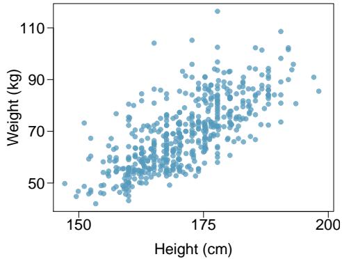
| Estimate | Std. Error | t value | Pr(>|t|) | |
| (Intercept) | -105.0113 | 7.5394 | -13.93 | 0.0000 |
| height | 1.0176 | 0.0440 | 23.13 | 0.0000 |
(a) Describe the relationship between height and weight.
(b) Write the equation of the regression line. Interpret the slope and intercept in context.
(c) Do the data provide strong evidence that an increase in height is associated with an increase in weight? State the null and alternative hypotheses, report the p-value, and state your conclusion.
(d) The correlation coefficient for height and weight is 0.72. Calculate \(R^2\) and interpret it in context.
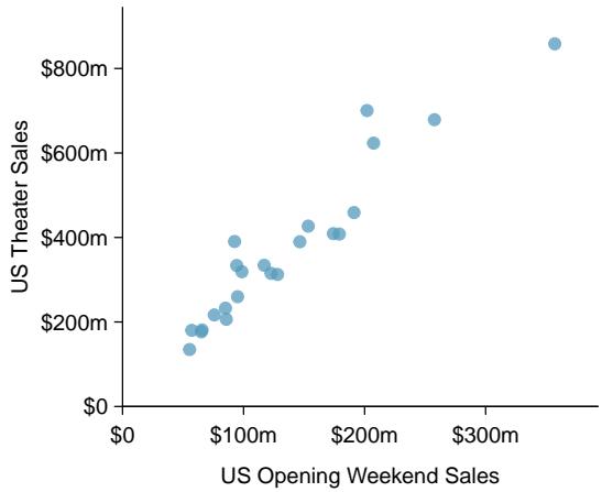
8.34 MCU, Predict US Theater Sales
The Marvel Comic Universe movies were an international movie sensation, containing 23 movies at the time of this writing. Here we consider a model predicting an MCU film's gross theater sales in the US based on the first weekend sales performance in the US.
| Estimate | Std. Error | t value | Pr(>|t|) | |
| (Intercept) | 42.5e6 | 26.6e6 | 1.60 | 0.1251 |
| opening_wednesday_us | 2.4361 | 0.1739 | 14.01 | 0.0000 |
(a) Describe the relationship between gross theater sales and first weekend sales.
(b) Write the equation of the regression line. Interpret the slope and intercept in context.
(c) Do the data provide strong evidence of an association? State hypotheses, report p-value, and conclude.
(d) The correlation is 0.950. Calculate \(R^2\) and interpret it.
(e) Would all films show as strong a relationship as MCU films?
8.35 Spouses, Part II
The scatterplot summarizes women's heights and their spouses' heights for a random sample of 170 married women in Britain.
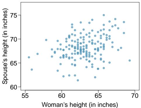
| Estimate | Std. Error | t value | Pr(>|t|) | |
| (Intercept) | 43.5755 | 4.6842 | 9.30 | 0.0000 |
| height_spouse | 0.2863 | 0.0686 | 4.17 | 0.0000 |
(a) Is there evidence that taller women have taller spouses? State hypotheses and test.
(b) Write the regression equation for predicting spouse's height.
(c) Interpret the slope and intercept.
(d) Given \(R^2 = 0.09\), what is the correlation?
(e) Predict the spouse's height for a woman who is 5'9" (69 inches). How reliable is this?
(f) Would you use this model to predict for a woman who is 6'7" (79 inches)? Why or why not?
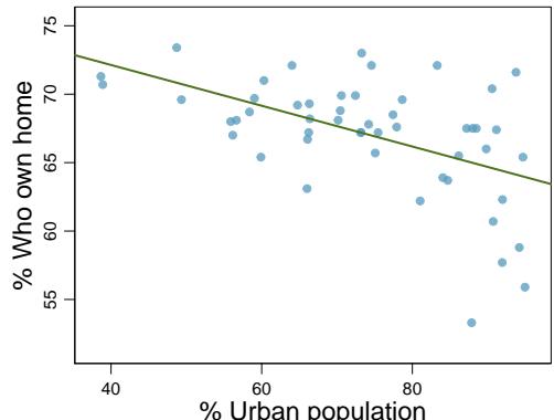
8.36 Urban Homeowners, Part II
For these data, \(R^2 = 0.28\).
(a) What is the correlation? How can you tell if it is positive or negative?
(b) Examine the residual plot. What do you observe? Is a simple least squares fit appropriate?
8.37 Murders and Poverty, Part II
| Estimate | Std. Error | t value | Pr(>|t|) | |
| (Intercept) | -29.901 | 7.789 | -3.839 | 0.001 |
| poverty% | 2.559 | 0.390 | 6.562 | 0.000 |
\[s = 5.512 \quad R^2 = 70.52\% \quad R_{adj}^2 = 68.89\%\]
(a) State hypotheses for evaluating whether poverty percentage predicts murder rate.
(b) State the conclusion in context.
(c) Calculate a 95% confidence interval for the slope and interpret it.
(d) Do the hypothesis test and confidence interval agree? Explain.
8.38 Babies
Is gestational age useful in predicting head circumference at birth for low birth-weight babies? The estimated regression line is:
\[\widehat{head circumference} = 3.91 + 0.78 \times \text{gestational age}\]
The standard error for the coefficient is 0.35. Is there significant evidence of a positive linear association? Use the five-step framework.
Chapter 8 Exercises
Practice problems to reinforce your understanding of linear regression concepts.
Why practice? These exercises test your understanding of correlation, regression, and inference. Working through them solidifies concepts and prepares you for assessments.
8.39 True / False
Determine if the following statements are true or false. If false, explain why.
(a) A correlation coefficient of -0.90 indicates a stronger linear relationship than a correlation of 0.5.
Answer: TRUE. The strength of correlation is measured by absolute value. |-0.90| = 0.90 > 0.5, so -0.90 indicates a stronger linear relationship.
(b) Correlation is a measure of the association between any two variables.
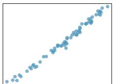
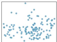
Answer: FALSE. Correlation measures linear association. It can miss strong nonlinear relationships (as shown in Figure 8.10).
8.40 Cats, Part II
Exercise 8.26 presents regression output from a model for predicting the heart weight (in g) of cats from their body weight (in kg). The coefficients are estimated using a dataset of 144 domestic cat. The model output is also provided below. Assume that conditions for inference on the slope are met.
| Estimate | Std. Error | t value | Pr(>|t|) | |
| (Intercept) | -0.357 | 0.692 | -0.515 | 0.607 |
| body wt | 4.034 | 0.250 | 16.119 | 0.000 |
\[s = 1.452 \quad R^{2} = 64.66\% \quad R_{adj}^{2} = 64.41\%\]
(a) What are the hypotheses for evaluating whether body weight is associated with heart weight in cats?
Answer: \(H_0: \beta = 0\) (no linear relationship) vs. \(H_A: \beta \neq 0\) (there is a linear relationship)
(b) State the conclusion of the hypothesis test from part (a) in context of the data.
Answer: With t = 16.119 and p < 0.001, we reject \(H_0\). There is very strong evidence of a positive linear relationship between body weight and heart weight in cats.
(c) Calculate a \(95\%\) confidence interval for the slope of body weight, and interpret it in context of the data.
Answer: $4.034 \pm 1.976 \times 0.250 = (3.54, 4.53)$. We are 95% confident that for each additional kg of body weight, heart weight increases by 3.54 to 4.53 grams on average.
(d) Do your results from the hypothesis test and the confidence interval agree? Explain.
Answer: Yes. The hypothesis test rejects \(\beta = 0\), and the confidence interval (3.54, 4.53) does not include 0, both indicating a significant positive relationship.
8.41 Nutrition at Starbucks, Part II
Exercise 8.22 introduced a data set on nutrition information on Starbucks food menu items. Based on the scatterplot and the residual plot provided, describe the relationship between the protein content and calories of these menu items, and determine if a simple linear model is appropriate to predict amount of protein from the number of calories.

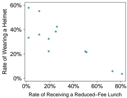
8.42 Helmets and Lunches
The scatterplot shows the relationship between socioeconomic status measured as the percentage of children in a neighborhood receiving reduced-fee lunches at school (lunch) and the percentage of bike riders in the neighborhood wearing helmets (helmet). The average percentage of children receiving reduced-fee lunches is $30.8\%\( with a standard deviation of \)26.7\%\( and the average percentage of bike riders wearing helmets is \)38.8\%\( with a standard deviation of \)16.9\%$.
(a) If the \(R^{2}\) for the least-squares regression line for these data is \(72\%\), what is the correlation between lunch and helmet?
(b) Calculate the slope and intercept for the least-squares regression line for these data.
(c) Interpret the intercept of the least-squares regression line in the context of the application.
(d) Interpret the slope of the least-squares regression line in the context of the application.
(e) What would the value of the residual be for a neighborhood where \(40\%\) of the children receive reduced-fee lunches and 40% of the bike riders wear helmets? Interpret the meaning of this residual in the context of the application.
8.43 Match the Correlation, Part III
Match each correlation to the corresponding scatterplot.
(a) \(r = -0.72\) (b) \(r = 0.07\) (c) \(r = 0.86\) (d) \(r = 0.99\)
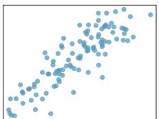 (1)
(1)
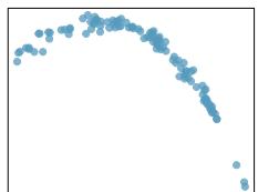 (2)
(2)
 (3)
(3)
 (4)
(4)
8.44 Rate My Professor
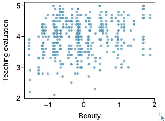
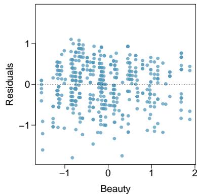
Many college courses conclude by giving students the opportunity to evaluate the course and the instructor anonymously. However, the use of these student evaluations as an indicator of course quality and teaching effectiveness is often criticized because these measures may reflect the influence of non-teaching related characteristics, such as the physical appearance of the instructor. Researchers at University of Texas, Austin collected data on teaching evaluation score (higher score means better) and standardized beauty score (a score of 0 means average, negative score means below average, and a positive score means above average) for a sample of 463 professors. The scatterplot below shows the relationship between these variables, and regression output is provided for predicting teaching evaluation score from beauty score.
| Estimate | Std. Error | t value | Pr(>|t|) | |
| (Intercept) | 4.010 | 0.0255 | 157.21 | 0.0000 |
| beauty | □ | 0.0322 | 4.13 | 0.0000 |
(a) Given that the average standardized beauty score is -0.0883 and average teaching evaluation score is 3.9983, calculate the slope. Alternatively, the slope may be computed using just the information provided in the model summary table.
(b) Do these data provide convincing evidence that the slope of the relationship between teaching evaluation and beauty is positive? Explain your reasoning.
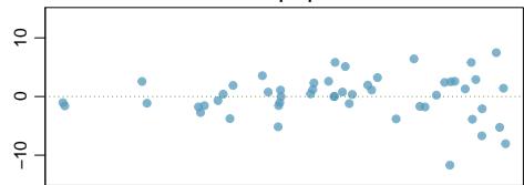
(c) List the conditions required for linear regression and check if each one is satisfied for this model based on the following diagnostic plots.
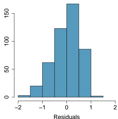
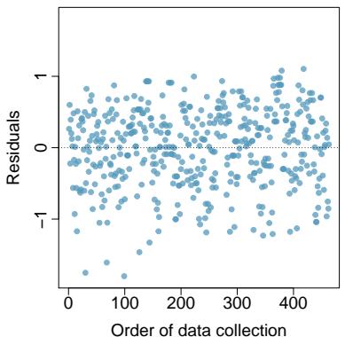
8.45 Trees
The scatterplots below show the relationship between height, diameter, and volume of timber in 31 felled black cherry trees. The diameter of the tree is measured 4.5 feet above the ground.
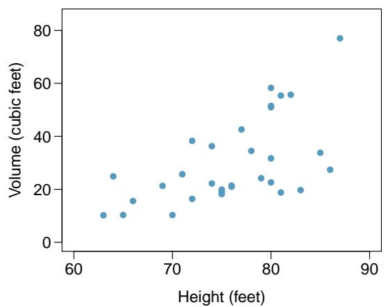
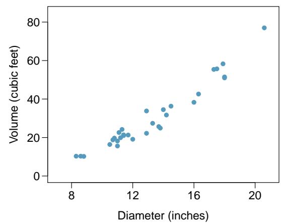
(a) Describe the relationship between volume and height of these trees.
(b) Describe the relationship between volume and diameter of these trees.
(c) Suppose you have height and diameter measurements for another black cherry tree. Which of these variables would be preferable to use to predict the volume of timber in this tree using a simple linear regression model? Explain your reasoning.