A.3 Poisson Distribution
Learning Objectives
By the end of this section, you will be able to:
- recognize when a counting problem is a Poisson setting, and name the interval the count is attached to;
- convert a stated average rate to the mean \(\mu\) for whatever interval the question actually asks about;
- compute \(P(X = x)\), \(P(X \le x)\), and "more than" probabilities for a Poisson random variable;
- find the mean and standard deviation of a Poisson distribution and say in plain words what each one measures;
- decide when the Poisson may stand in for the binomial, and carry out the approximation.
A.3.1 What Makes an Experiment Poisson
A Poisson experiment gives the probability of a number of events occurring in a fixed interval of time or space, when
- the events happen at a known average rate, and
- the events happen independently of the time since the last event.
Change "typos per 100 pages" to "typos per page" and you have a different random variable with a different mean, even though nothing about the book changed. Name the interval first, then find the average for THAT interval, then ask the probability question.
The random variable \(X\) counts the number of occurrences in the interval of interest, so \(X\) takes on the values \(x = 0, 1, 2, 3, \ldots\) with no fixed upper bound.
Take the book editor. On average there are five words spelled incorrectly in 100 pages. The interval is the 100 pages. The count is however many typos actually turn up in a particular 100 pages — it could be two, it could be eleven, and there is no ceiling on it the way a binomial's \(n\) is a ceiling.
That second characteristic is the one people skip past, so it is worth saying in plain words. Independence here means the clock does not remember. If a typo showed up on page 3, that tells you nothing about whether one shows up on page 4. If the ER has been quiet for forty minutes, that does not make a patient "due." Every stretch of the interval carries the same rate as every other stretch, and nothing that already happened changes it.
Two more things follow from the definition. The count is discrete — you can have three typos or four, never 3.5. And the distribution has no upper limit, which is why "more than" questions in this section always get answered through their complement rather than by adding up an endless tail. Both of these will matter in the very first example.
A Poisson experiment has two defining characteristics, and the first one is the one that decides whether the distribution applies at all.
A Poisson experiment counts the events that land inside one fixed interval.
The average number of fish caught in an hour is eight. Of interest is the number of fish caught in 15 minutes. The time interval of interest is 15 minutes. What is the average number of fish caught in 15 minutes?
Solution
Step 1 — Compare the two intervals. The rate you are given is per hour. The interval you want is 15 minutes, which is \(\frac{1}{4}\) of an hour.
Step 2 — Scale the rate by the same fraction.
$$\left(\frac{1}{4}\right)(8) = 2$$Answer: 2 fish, on average, in a 15-minute interval.
The average number of loaves of bread put on a shelf in a bakery in a half-hour period is 12. Of interest is the number of loaves of bread put on the shelf in five minutes. The time interval of interest is five minutes. What is the probability that the number of loaves, selected randomly, put on the shelf in five minutes is three?
Solution
Step 1 — Name the random variable. Let \(X\) be the number of loaves of bread put on the shelf in five minutes.
Step 2 — Scale the average to the interval you were asked about. The average is given for 30 minutes, but the question asks about five minutes, which is \(\frac{5}{30}\) of that.
$$\left(\frac{5}{30}\right)(12) = 2 \text{ loaves of bread}$$So \(\mu = 2\) for this problem.
Step 3 — Write the probability question. The question asks you to find \(P(x = 3)\).
Step 4 — Evaluate it. Using the Poisson probability formula from the next subsection with \(\mu = 2\) and \(x = 3\):
$$P(x = 3) = \frac{2^{3}e^{-2}}{3!} = \frac{(8)(0.1353)}{6} \approx 0.1804$$Answer: about a 0.1804 chance, or roughly 18%, that exactly three loaves go on the shelf in a given five-minute stretch.
An electronics store expects to have ten returns per day on average. The manager wants to know the probability of the store getting fewer than eight returns on any given day. State the probability question mathematically.
Solution
Step 1 — Name the random variable and the interval. Let \(X\) be the number of returns the store gets in one day. The interval of interest is one day, and the average for that interval is \(\mu = 10\).
Step 2 — Translate "fewer than eight." Fewer than eight means eight is excluded, so the values that count are 0 through 7.
Answer: \(P(x < 8)\), which is the same as \(P(x \le 7)\). Evaluating it gives \(P(x \le 7) = \text{poissoncdf}(10, 7) \approx 0.2202\).
A bank expects to receive six bad checks per day, on average. What is the probability of the bank getting fewer than five bad checks on any given day? Of interest is the number of checks the bank receives in one day, so the time interval of interest is one day. Let \(X\) be the number of bad checks the bank receives in one day. If the bank expects to receive six bad checks per day then the average is six checks per day. Write a mathematical statement for the probability question.
Solution
Step 1 — Confirm the mean matches the interval. The rate and the interval are already the same — six per day, asked about one day — so no scaling is needed and \(\mu = 6\).
Step 2 — Translate the words into symbols. "Fewer than five" excludes five itself, so the values that count are 0, 1, 2, 3, and 4.
$$P(x < 5)$$Answer: the mathematical statement is \(P(x < 5)\). Since \(X\) is discrete, this is the same as \(P(x \le 4)\), which evaluates to \(\text{poissoncdf}(6, 4) \approx 0.2851\).
An emergency room at a particular hospital gets an average of five patients per hour. A doctor wants to know the probability that the ER gets more than five patients per hour. Give the reason why this would be a Poisson distribution.
Solution
Step 1 — Check the interval. There is a fixed interval of time — one hour — and a known average rate for it, five patients.
Step 2 — Check independence. One patient walking in does not change the chance that another walks in a minute later. Arrivals at an ER are unrelated to each other.
Step 3 — Check the count. \(X\) counts occurrences in that interval and could be any whole number: 0, 1, 2, and so on, with no fixed maximum.
Answer: it is a Poisson setting because the count is of events in a fixed interval, the events occur at a known average rate, and each arrival is independent of the time since the last one. (The probability itself is \(P(x > 5) = 1 - \text{poissoncdf}(5, 5) \approx 0.3840\).)
You notice that Dana Whitfield, a local news anchor, says "uh," on average, two times per broadcast. What is the probability that she says "uh" more than two times per broadcast?
This is a Poisson problem because you are interested in knowing the number of times she says "uh" during a broadcast.
a. What is the interval of interest?
b. What is the average number of times she says "uh" during one broadcast?
c. Let \(X = \) _______. What values does \(X\) take on?
d. The probability question is \(P(\_\_\_\_\_\_)\).
Solution
a. The interval. One broadcast. Notice the interval here is not a stretch of clock time at all — it is one unit of a repeatable thing, and that works exactly the same way.
b. The average for that interval. 2.
c. The random variable. Let \(X\) be the number of times she says "uh" during one broadcast. Then
$$x = 0, 1, 2, 3, \ldots$$The reporter could get through a broadcast without saying it once, or say it many times, so there is no upper bound to list.
d. The probability question.
$$P(x > 2)$$Answer: interval = one broadcast, \(\mu = 2\), \(x = 0, 1, 2, 3, \ldots\), and the question is \(P(x > 2)\). Evaluating it: \(P(x > 2) = 1 - P(x \le 2) = 1 - \text{poissoncdf}(2, 2) \approx 0.3233\).
A.3.2 Notation and the Poisson Formula
The notation
$$X \sim P(\mu)$$is read "\(X\) is a random variable with a Poisson distribution." The parameter is \(\mu\) (or \(\lambda\)), where \(\mu\) is the mean for the interval of interest. The standard deviation of a Poisson distribution with mean \(\mu\) is
$$\sigma = \sqrt{\mu}$$With no fixed \(n\) and no per-trial \(p\), there is nothing left to describe the distribution except how busy the interval is on average. Tell me the rate and I can tell you the whole shape.
One parameter is all it takes. The binomial needed \(n\) and \(p\); the hypergeometric needed three numbers. The Poisson needs only the average count for the interval, and everything else — every individual probability, the spread — follows from it. That is also why the standard deviation formula looks so bare: the variance of a Poisson distribution is \(\sigma^2 = \mu\), the mean and the variance are the same number, so the standard deviation is just its square root.
The formula below is what actually produces each probability. You will mostly evaluate it with technology, but it is worth reading once for what it says: the chance of exactly \(x\) events is the mean raised to the \(x\), damped by \(e^{-\mu}\), divided by the number of ways \(x\) things can be ordered.
One parameter sets the whole shape: raising the mean walks the bars off the wall at zero.
If \(X \sim P(\mu)\), the probability of exactly \(x\) occurrences in the interval of interest is
$$P(X = x) = \frac{\mu^{x}e^{-\mu}}{x!}$$where \(x = 0, 1, 2, 3, \ldots\) and \(x!\) is \(x\) factorial.
One consequence shows up in almost every problem in this section. Because the Poisson runs through every whole number with no ceiling, a question like "more than one" covers infinitely many values and cannot be added up directly. The way around it is the complement: subtract the short side from 1. "More than one" is everything except zero and one, so \(P(x > 1) = 1 - [P(x = 0) + P(x = 1)]\). The next example runs that move end to end.
Every distribution in this chapter has a shorthand, and the Poisson's is the shortest of them all, because it takes only one number.
A customer service center receives about ten emails every half-hour. What is the probability that the customer service center receives more than four emails in the next six minutes?
Solution
Step 1 — Scale the rate to the interval asked about. Six minutes is \(\frac{6}{30} = \frac{1}{5}\) of a half-hour, so
$$\mu = \left(\frac{1}{5}\right)(10) = 2 \text{ emails}$$Step 2 — Write the question and flip to the complement. "More than four" means \(x = 5, 6, 7, \ldots\), which never ends, so subtract the short side instead:
$$P(x > 4) = 1 - P(x \le 4)$$Step 3 — Evaluate.
$$P(x > 4) = 1 - \text{poissoncdf}(2, 4) = 1 - 0.9473 \approx 0.0527$$Answer: about 0.0527, so a little over a 5% chance of more than four emails in a six-minute stretch.
Thao Vang receives about six telephone calls between 8 a.m. and 10 a.m. What is the probability that he receives more than one call in the next 15 minutes?
Solution
Step 1 — Name the random variable and the interval. Let \(X\) be the number of calls Thao receives in 15 minutes. The interval of interest is 15 minutes, or \(\frac{1}{4}\) hour, and
$$x = 0, 1, 2, 3, \ldots$$Step 2 — Scale the average. He receives six calls in two hours, and there are eight 15-minute intervals in two hours, so
$$\left(\frac{1}{8}\right)(6) = 0.75 \text{ calls in 15 minutes, on average}$$So \(\mu = 0.75\) for this problem.
Step 3 — Flip "more than one" to its complement. The Poisson distribution is discrete, and \(x > 1\) includes all whole numbers through infinity. The way to handle that is to subtract the probability of one or fewer:
$$P(x > 1) = 1 - P(x \le 1) = 1 - [P(x = 0) + P(x = 1)]$$Step 4 — Evaluate both terms with the formula.
$$ \begin{aligned} P(x > 1) &= 1 - \left[\frac{0.75^{0}e^{-0.75}}{0!} + \frac{0.75^{1}e^{-0.75}}{1!}\right] \\ &= 1 - \left[\frac{(1)(0.4724)}{1} + \frac{(0.75)(0.4724)}{1}\right] \\ &= 1 - [0.4724 + 0.3543] = 0.1733 \end{aligned} $$Answer: \(P(x > 1) \approx 0.1733\), a little under a 1-in-5 chance. (Cumulative technology reports 0.1734; the difference is rounding in the two hand-computed terms.)
Let the tool take the complement for you
You do not need a graphing calculator for this. In rāSHio, choose Distributions → Poisson and set the mean to 0.75 — the panel calls it \(\lambda\), which is the same number this book calls \(\mu\). Then pick Right and enter \(k = 2\), because "more than one" is "two or more" once the values are whole numbers. It returns 0.1734 directly, so the two-term subtraction in Step 4 above becomes a check rather than the work.
Figure A.3.1 — The rāSHio Poisson panel: Distributions → Poisson. Set the mean, pick a region, read the probability. The walkthrough uses its own demonstration numbers, not this section's.
The picture below is what those numbers look like laid out side by side. Each bar is one value of \(x\), and its height is the probability of that many calls. Notice how fast the bars fall off: with a mean of only 0.75 calls per quarter hour, zero calls is by far the most likely outcome, and everything past three is small enough to lump into "etc."
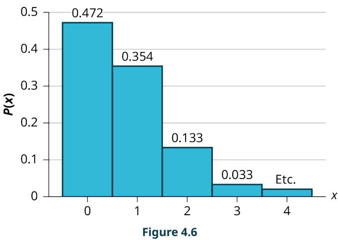
Figure A.3.2 — Poisson probabilities for the number of calls Thao receives in 15 minutes, with a mean of 0.75 calls.
The vertical axis in Figure A.3.2 contains the probability of \(x\), where \(X\) is the number of calls in 15 minutes.
A.3.3 Changing the Interval, and Large Means
The two examples in this subsection both hinge on the same move — take a rate quoted for one interval and restate it for the interval the question actually asks about — but they push it in opposite directions. One scales a daily rate up into a mean of 147; the other scales a daily rate down to an hourly one. Getting \(\mu\) matched to the interval is most of the work in a Poisson problem, and once it is right the rest is one function call.
Large means are worth a word on their own. Nothing in the formula cares whether \(\mu\) is 0.75 or 187, but the shape of the distribution changes a lot. With a small mean the bars pile up against zero and fall off fast, as they did in Figure A.3.2. With a large mean the bars spread into a mound centered near \(\mu\), and a value 12 away from the mean stops being remarkable. The standard deviation \(\sigma = \sqrt{\mu}\) is what quantifies that: at \(\mu = 147\) the spread is about 12, so 160 is only about one standard deviation above average.
According to a recent poll by the Pew Internet Project, people between the ages of 14 and 17 send an average of 187 text messages each day. Let \(X\) be the number of texts that a person aged 14 to 17 sends per day. The discrete random variable \(X\) takes on the values \(x = 0, 1, 2, \ldots\). The random variable \(X\) has a Poisson distribution: \(X \sim P(187)\). The mean is 187 text messages.
a. What is the probability that a person sends exactly 175 texts per day?
b. What is the probability that a person sends at most 150 texts per day?
c. What is the standard deviation?
Solution
a. Exactly 175. "Exactly" means a single value, so this is the probability density function:
$$P(x = 175) = \text{poissonpdf}(187, 175) \approx 0.0203$$b. At most 150. "At most" includes 150 itself, so it is cumulative:
$$P(x \le 150) = \text{poissoncdf}(187, 150) \approx 0.0030$$That is a small number, and the reason is the spread — 150 is nearly three standard deviations below the mean.
c. The standard deviation.
$$\sigma = \sqrt{\mu} = \sqrt{187} \approx 13.6748$$Answer: a. 0.0203 b. 0.0030 c. about 13.6748 texts.
According to Baydin, an email management company, an email user gets, on average, 147 emails per day. Let \(X\) be the number of emails an email user receives per day. The discrete random variable \(X\) takes on the values \(x = 0, 1, 2, \ldots\). The random variable \(X\) has a Poisson distribution: \(X \sim P(147)\). The mean is 147 emails.
a. What is the probability that an email user receives exactly 160 emails per day?
b. What is the probability that an email user receives at most 160 emails per day?
c. What is the standard deviation?
Solution
a. Exactly 160. A single value calls for the probability density function:
$$P(x = 160) = \text{poissonpdf}(147, 160) \approx 0.0180$$b. At most 160. "At most" sweeps up everything from 0 through 160, so it is cumulative:
$$P(x \le 160) = \text{poissoncdf}(147, 160) \approx 0.8666$$c. The standard deviation.
$$\sigma = \sqrt{\mu} = \sqrt{147} \approx 12.1244$$Answer: a. 0.0180 b. 0.8666 c. about 12.1244 emails. Part b is worth reading against part c: 160 sits about one standard deviation above the mean, and roughly 87% of days come in at or below it.
Atlanta's Hartsfield-Jackson International Airport is the busiest airport in the world. On average there are 2,700 arrivals and departures each day.
a. How many airplanes arrive and depart the airport per hour?
b. What is the probability that there are exactly 100 arrivals and departures in one hour?
c. What is the probability that there are at most 100 arrivals and departures in one hour?
Solution
a. Rescale the daily rate to an hour. There are 24 hours in a day:
$$\mu = \frac{2{,}700}{24} = 112.5 \text{ arrivals and departures per hour}$$b. Exactly 100.
$$P(x = 100) = \text{poissonpdf}(112.5, 100) \approx 0.0194$$c. At most 100.
$$P(x \le 100) = \text{poissoncdf}(112.5, 100) \approx 0.1279$$Answer: a. 112.5 per hour b. 0.0194 c. 0.1279. A slow hour of 100 or fewer movements happens about 13% of the time.
Text message users receive or send an average of 41.5 text messages per day.
a. How many text messages does a text message user receive or send per hour?
b. What is the probability that a text message user receives or sends two messages per hour?
c. What is the probability that a text message user receives or sends more than two messages per hour?
Solution
a. Rescale the daily rate to an hour. Let \(X\) be the number of texts that a user sends or receives in one hour. The average number of texts received per hour is
$$\frac{41.5}{24} \approx 1.7292$$b. Exactly two. With \(X \sim P(1.7292)\),
$$P(x = 2) = \text{poissonpdf}(1.7292, 2) \approx 0.2653$$c. More than two. Take the complement, as always with an open-ended upper tail:
$$P(x > 2) = 1 - P(x \le 2) = 1 - \text{poissoncdf}(1.7292, 2) \approx 1 - 0.7495 = 0.2505$$Answer: a. about 1.7292 texts per hour b. 0.2653 c. 0.2505.
A.3.4 Using the Poisson to Approximate the Binomial
When the number of trials \(n\) is large and the probability of success \(p\) is small, a binomial random variable \(X \sim B(n, p)\) is well approximated by a Poisson random variable with
$$\mu = np$$where \(n\) is the number of independent trials and \(p\) is the probability of success on a single trial. The usual working guideline is \(n \ge 20\) and \(p \le 0.05\).
Defective bulbs in a string of 100, audited returns among 100 filers, extra fortunes in a bag of 144 cookies — all are "many chances, small odds," which is the shape the Poisson approximates best.
The two thresholds do different jobs. A large \(n\) is what lets a bounded count behave like an unbounded one — with 200 trials, the difference between "at most 200 successes" and "no ceiling" is invisible in the region where the probability actually lives. A small \(p\) is what keeps the mean modest even though \(n\) is big, which is exactly the regime the Poisson was built for. When both hold, the two distributions give answers that agree to several decimal places, and you get to trade three parameters for one.
The second characteristic named at the top of this section is the one we have not used yet: the Poisson distribution may be used to approximate the binomial. This matters when \(n\) is large enough that binomial arithmetic gets unwieldy, and it works because a binomial with many trials and a tiny success probability behaves almost exactly like a Poisson with the same average number of successes.
Hold np fixed and raise n: the binomial bars settle onto their Poisson stand-in.
On a certain day in May starting at 4:30 PM, the probability of moderate seismic activity for the next 48 hours in the Kuril Islands off the coast of Japan was reported at about 1.43%. Use this information for the next 100 days to find the probability that there will be moderate seismic activity in five of the next 100 days. Use both the binomial and Poisson distributions to calculate the probabilities. Are they close?
Solution
Step 1 — Name the random variable. Let \(X\) be the number of days with moderate seismic activity out of 100.
Step 2 — Binomial. Here \(n = 100\) and \(p = 0.0143\):
$$P(x = 5) = \text{binompdf}(100, 0.0143, 5) \approx 0.0115$$Step 3 — Poisson. Compute the mean first:
$$\mu = np = 100(0.0143) = 1.43$$ $$P(x = 5) = \text{poissonpdf}(1.43, 5) \approx 0.0119$$Step 4 — Check the guideline. \(n = 100 \ge 20\) and \(p = 0.0143 \le 0.05\), so the approximation should be good.
Answer: binomial \(\approx 0.0115\), Poisson \(\approx 0.0119\). Yes, they are close — they agree to two decimal places, and the small gap is what "approximation" costs you.
On a certain day in May starting at 4:30 PM, the probability of low seismic activity for the next 48 hours in Alaska was reported as about 1.02%. Use this information for the next 200 days to find the probability that there will be low seismic activity in ten of the next 200 days. Use both the binomial and Poisson distributions to calculate the probabilities. Are they close?
Solution
Step 1 — Name the random variable. Let \(X\) be the number of days with low seismic activity.
Step 2 — Using the binomial distribution. Each of the 200 days is a trial with \(p = 0.0102\):
$$P(x = 10) = \text{binompdf}(200, 0.0102, 10) \approx 0.000039$$Step 3 — Using the Poisson distribution. Calculate the mean:
$$\mu = np = 200(0.0102) \approx 2.04$$ $$P(x = 10) = \text{poissonpdf}(2.04, 10) \approx 0.000045$$Step 4 — Compare. We expect the approximation to be good because \(n\) is large (greater than 20) and \(p\) is small (less than 0.05).
Answer: the results are close — both probabilities reported are almost 0. Ten quiet days out of 200 is far above the mean of about two, so both distributions agree it essentially does not happen.
Run both sides of the comparison in one place
The two examples above ask you to compute a binomial probability and a Poisson one and then hold them side by side, and rāSHio does both. For the binomial half, choose Calculators → Binomial, set Trials (n) to 200 and Success probability (p) to 0.0102, pick Exact, and enter 10 — it returns the 0.000039 this example reports. Then switch to Distributions → Poisson with a mean of 2.04 for the other half. Doing it twice is the point: the guideline is only worth trusting once you have watched the two answers land on top of each other.
Figure A.3.3 — The rāSHio Binomial Calculator: Calculators → Binomial. One panel, four tabs — Exact, At Most, At Least, Range. The walkthrough uses its own demonstration numbers, not this section's.
Problem Set A.3
Use the following information to answer the next six exercises: On average, a clothing store gets 120 customers per day.
Problem 1. Assume the event occurs independently in any given day. Define the random variable \(X\).
Solution
Step 1 — Find the interval. The rate you are given is 120 customers per day, and the exercise asks about a day, so the interval of interest is one day.
Step 2 — Say what is being counted. \(X\) counts occurrences in that interval.
Answer: \(X\) = the number of customers the clothing store gets in one day.
Problem 2. What values does \(X\) take on?
Solution
Step 1 — Recall the range of a Poisson variable. A Poisson count starts at zero and has no fixed upper bound — there is no \(n\) capping it the way a binomial has.
Answer: \(x = 0, 1, 2, 3, \ldots\)
Problem 3. What is the probability of getting 150 customers in one day?
Solution
Step 1 — Match the mean to the interval. The question asks about one day, and the average for one day is already given, so \(\mu = 120\) and \(X \sim P(120)\).
Step 2 — "Getting 150 customers" is a single value, so use the probability density function.
$$P(x = 150) = \text{poissonpdf}(120, 150) \approx 0.0010$$Answer: about 0.0010. With a standard deviation of \(\sqrt{120} \approx 10.95\), a day of 150 sits nearly three standard deviations above average, which is why it is so unlikely.
Problem 4. What is the probability of getting 35 customers in the first four hours? Assume the store is open 12 hours each day.
Solution
Step 1 — Rescale to an hourly rate. The store is open 12 hours and averages 120 customers, so it averages \(\frac{120}{12} = 10\) customers per hour.
Step 2 — Scale up to the interval asked about. Four hours gives
$$\mu = 4(10) = 40 \text{ customers}$$Step 3 — Evaluate.
$$P(x = 35) = \text{poissonpdf}(40, 35) \approx 0.0485$$Answer: about 0.0485.
Problem 5. What is the probability that the store will have more than 12 customers in the first hour?
Solution
Step 1 — Set the mean for one hour. From the previous problem, the store averages 10 customers per hour, so \(\mu = 10\).
Step 2 — Flip "more than 12" to its complement. The upper tail runs forever, so subtract the short side.
$$P(x > 12) = 1 - P(x \le 12) = 1 - \text{poissoncdf}(10, 12) \approx 1 - 0.7916 = 0.2084$$Answer: about 0.2084, so a busier-than-12 first hour happens roughly one day in five.
Problem 6. What is the probability that the store will have fewer than 12 customers in the first two hours?
Solution
Step 1 — Scale to two hours. At 10 customers per hour, two hours gives \(\mu = 20\).
Step 2 — Translate "fewer than 12." Fewer than 12 excludes 12 itself, so the values that count are 0 through 11.
$$P(x < 12) = P(x \le 11) = \text{poissoncdf}(20, 11) \approx 0.0214$$Answer: about 0.0214 — a very quiet two hours.
Problem 7. Which type of distribution can the Poisson model be used to approximate? When would you do this?
Solution
Step 1 — Name the distribution. The Poisson can stand in for the binomial.
Step 2 — Say when. Use it when the number of trials \(n\) is large and the probability of success \(p\) on a single trial is small — the working guideline in this section is \(n \ge 20\) and \(p \le 0.05\). Set the Poisson mean to \(\mu = np\).
Answer: the binomial distribution, when \(n\) is large (\(n \ge 20\)) and \(p\) is small (\(p \le 0.05\)); then \(B(n, p)\) is well approximated by \(P(np)\).
Use the following information to answer the next six exercises: On average, eight teens in the U.S. die from motor vehicle injuries per day. As a result, states across the country are debating raising the driving age.
Problem 8. Assume the event occurs independently in any given day. In words, define the random variable \(X\).
Solution
Step 1 — Find the interval. The rate is eight per day and the exercise asks about any given day, so the interval of interest is one day.
Answer: \(X\) = the number of U.S. teens who die from motor vehicle injuries in one day.
Problem 9. Give the distribution of \(X\). \(X \sim\) _______(_______)
Solution
Step 1 — Identify the parameter. A Poisson distribution takes one number, the mean for the interval of interest, which here is 8.
Answer: \(X \sim P(8)\).
Problem 10. What values does \(X\) take on?
Solution
Answer: \(x = 0, 1, 2, 3, \ldots\) — every whole number, with no upper bound.
Problem 11. For \(x = 0, 1, 2, 3, 4,\) and 5, find the corresponding probabilities \(P(x)\).
Solution
Step 1 — Use the Poisson formula with \(\mu = 8\).
$$P(x) = \frac{8^{x}e^{-8}}{x!}$$Step 2 — Evaluate at each value.
| x | P(x) |
|---|---|
| 0 | 0.0003 |
| 1 | 0.0027 |
| 2 | 0.0107 |
| 3 | 0.0286 |
| 4 | 0.0573 |
| 5 | 0.0916 |
Answer: the probabilities rise steadily across this range because all six values are still below the mean of 8 — the peak of the distribution is out at \(x = 7\) and \(x = 8\).
Problem 12. Is it likely that there will be no teens killed from motor vehicle injuries on any given day in the U.S.? Justify your answer numerically.
Solution
Step 1 — Translate "no teens killed" into a probability. That is exactly \(P(x = 0)\) with \(\mu = 8\).
$$P(x = 0) = \frac{8^{0}e^{-8}}{0!} = e^{-8} \approx 0.0003$$Step 2 — Judge the number. A probability of 0.0003 is about 3 chances in 10,000, or roughly one such day every nine years.
Answer: no, it is not likely. \(P(x = 0) \approx 0.0003\), which is small enough that a day with zero deaths would be a genuinely rare event.
Problem 13. Is it likely that there will be more than 20 teens killed from motor vehicle injuries on any given day in the U.S.? Justify your answer numerically.
Solution
Step 1 — Flip to the complement.
$$P(x > 20) = 1 - P(x \le 20) = 1 - \text{poissoncdf}(8, 20) \approx 1 - 0.9999 = 0.0001$$Step 2 — Judge the number. With a mean of 8 and a standard deviation of \(\sqrt{8} \approx 2.83\), the value 21 sits more than four standard deviations above average.
Answer: no. \(P(x > 20) \approx 0.0001\), about one chance in 10,000, so more than 20 deaths in a single day would be far outside the normal range.
Problem 14. The switchboard in a Minneapolis law office gets an average of 5.5 incoming phone calls during the noon hour on Mondays. Experience shows that the existing staff can handle up to six calls in an hour. Let \(X\) be the number of calls received at noon.
a) Find the mean and standard deviation of \(X\).
b) What is the probability that the office receives at most six calls at noon on Monday?
c) Find the probability that the law office receives six calls at noon. What does this mean to the law office staff who get, on average, 5.5 incoming phone calls at noon?
d) What is the probability that the office receives more than eight calls at noon?
Solution
a. Mean and standard deviation. The interval is the noon hour and the average for it is 5.5 calls, so \(X \sim P(5.5)\), and
$$\mu = 5.5 \qquad \sigma = \sqrt{\mu} = \sqrt{5.5} \approx 2.3452$$b. At most six calls. "At most" includes six, so it is cumulative.
$$P(x \le 6) = \text{poissoncdf}(5.5, 6) \approx 0.6860$$c. Exactly six calls.
$$P(x = 6) = \text{poissonpdf}(5.5, 6) \approx 0.1571$$To the staff, that means about 16% of Mondays land exactly at the limit of what they can handle. Read alongside part b, it also says the office is over its limit on the other \(1 - 0.6860 = 0.3140\), or about 31%, of Mondays — roughly one Monday in three.
d. More than eight calls.
$$P(x > 8) = 1 - P(x \le 8) = 1 - \text{poissoncdf}(5.5, 8) \approx 1 - 0.8944 = 0.1056$$Answer: a. \(\mu = 5.5\), \(\sigma \approx 2.3452\) b. 0.6860 c. 0.1571, and the office is over capacity about 31% of Mondays d. 0.1056.
Problem 15. The maternity ward at Dr. Jose Fabella Memorial Hospital in Manila in the Philippines is one of the busiest in the world with an average of 60 births per day. Let \(X\) be the number of births in an hour.
a) Find the mean and standard deviation of \(X\).
b) Sketch a graph of the probability distribution of \(X\).
c) What is the probability that the maternity ward will deliver three babies in one hour?
d) What is the probability that the maternity ward will deliver at most three babies in one hour?
e) What is the probability that the maternity ward will deliver more than five babies in one hour?
Solution
a. Mean and standard deviation. The ward averages 60 births per day, and the interval asked about is one hour, so scale by \(\frac{1}{24}\):
$$\mu = \frac{60}{24} = 2.5 \text{ births per hour} \qquad \sigma = \sqrt{2.5} \approx 1.5811$$b. The graph. Plot \(x\) on the horizontal axis and \(P(x)\) on the vertical axis, one bar per value. With \(\mu = 2.5\) the bars rise to a peak at \(x = 2\) (0.2565), sit nearly level at \(x = 3\) (0.2138), and fall off steadily after that — the same shape as Figure A.3.2, just shifted right and less lopsided because the mean is larger.
c. Exactly three births.
$$P(x = 3) = \text{poissonpdf}(2.5, 3) \approx 0.2138$$d. At most three births.
$$P(x \le 3) = \text{poissoncdf}(2.5, 3) \approx 0.7576$$e. More than five births.
$$P(x > 5) = 1 - P(x \le 5) = 1 - \text{poissoncdf}(2.5, 5) \approx 1 - 0.9580 = 0.0420$$Answer: a. \(\mu = 2.5\), \(\sigma \approx 1.5811\) b. a right-skewed bar graph peaking at \(x = 2\) c. 0.2138 d. 0.7576 e. 0.0420.
Problem 16. A manufacturer of Christmas tree light bulbs knows that 3% of its bulbs are defective. Find the probability that a string of 100 lights contains at most four defective bulbs using both the binomial and Poisson distributions.
Solution
Step 1 — Name the random variable. Let \(X\) be the number of defective bulbs in a string of 100.
Step 2 — Using the Poisson distribution. With \(n = 100\) and \(p = 0.03\),
$$\mu = np = 100(0.03) = 3 \qquad X \sim P(3)$$ $$P(x \le 4) = \text{poissoncdf}(3, 4) \approx 0.8153$$Step 3 — Using the binomial distribution. With \(X \sim B(100, 0.03)\),
$$P(x \le 4) = \text{binomcdf}(100, 0.03, 4) \approx 0.8179$$Step 4 — Compare. The guideline holds — \(n = 100 \ge 20\) and \(p = 0.03 \le 0.05\) — so the two answers should agree closely, and they differ by only about 0.003.
Answer: Poisson \(\approx 0.8153\), binomial \(\approx 0.8179\).
Problem 17. The average number of children a Japanese woman has in her lifetime is 1.37. Suppose that one Japanese woman is randomly chosen.
a) In words, define the random variable \(X\).
b) List the values that \(X\) may take on.
c) Give the distribution of \(X\). \(X \sim\) _______(_______)
d) Find the probability that she has no children.
e) Find the probability that she has fewer children than the Japanese average.
f) Find the probability that she has more children than the Japanese average.
Solution
a. \(X\) = the number of children a randomly chosen Japanese woman has in her lifetime.
b. \(x = 0, 1, 2, 3, \ldots\)
c. \(X \sim P(1.37)\).
d. No children.
$$P(x = 0) = e^{-1.37} \approx 0.2541$$e. Fewer children than the average. The average is 1.37, and \(X\) only takes whole-number values, so "fewer than 1.37" means \(x = 0\) or \(x = 1\).
$$P(x \le 1) = \text{poissoncdf}(1.37, 1) \approx 0.6022$$f. More children than the average. That is everything from 2 up, which is the complement of part e.
$$P(x \ge 2) = 1 - P(x \le 1) \approx 1 - 0.6022 = 0.3978$$Answer: a. the number of children a Japanese woman has b. \(0, 1, 2, 3, \ldots\) c. \(X \sim P(1.37)\) d. 0.2541 e. 0.6022 f. 0.3978.
Problem 18. The average number of children a Spanish woman has in her lifetime is 1.47. Suppose that one Spanish woman is randomly chosen.
a) In words, define the random variable \(X\).
b) List the values that \(X\) may take on.
c) Give the distribution of \(X\). \(X \sim\) _______(_______)
d) Find the probability that she has no children.
e) Find the probability that she has fewer children than the Spanish average.
f) Find the probability that she has more children than the Spanish average.
Solution
a. \(X\) = the number of children a randomly chosen Spanish woman has in her lifetime.
b. \(x = 0, 1, 2, 3, \ldots\)
c. \(X \sim P(1.47)\).
d. No children.
$$P(x = 0) = e^{-1.47} \approx 0.2299$$e. Fewer children than the average. Whole numbers below 1.47 are 0 and 1.
$$P(x \le 1) = \text{poissoncdf}(1.47, 1) \approx 0.5679$$f. More children than the average.
$$P(x \ge 2) = 1 - P(x \le 1) \approx 1 - 0.5679 = 0.4321$$Answer: a. the number of children a Spanish woman has b. \(0, 1, 2, 3, \ldots\) c. \(X \sim P(1.47)\) d. 0.2299 e. 0.5679 f. 0.4321.
Problem 19. Fertile, female cats produce an average of three litters per year. Suppose that one fertile, female cat is randomly chosen.
a) In words, define the random variable \(X\).
b) List the values that \(X\) may take on.
c) Give the distribution of \(X\). \(X \sim\) _______(_______)
d) Find the probability that she has no litters in one year.
e) Find the probability that she has at least two litters in one year.
f) Find the probability that she has exactly three litters in one year.
Solution
a. \(X\) = the number of litters a randomly chosen fertile female cat produces in one year.
b. \(x = 0, 1, 2, 3, \ldots\)
c. \(X \sim P(3)\).
d. No litters.
$$P(x = 0) = e^{-3} \approx 0.0498$$e. At least two litters. "At least two" is everything except 0 and 1.
$$P(x \ge 2) = 1 - P(x \le 1) \approx 1 - 0.1991 = 0.8009$$f. Exactly three litters.
$$P(x = 3) = \text{poissonpdf}(3, 3) \approx 0.2240$$Answer: a. the number of litters in one year b. \(0, 1, 2, 3, \ldots\) c. \(X \sim P(3)\) d. 0.0498 e. 0.8009 f. 0.2240.
Problem 20. The chance of having an extra fortune in a fortune cookie is about 3%. Given a bag of 144 fortune cookies, we are interested in the number of cookies with an extra fortune. Two distributions may be used to solve this problem, but only use one distribution to solve the problem.
a) In words, define the random variable \(X\).
b) List the values that \(X\) may take on.
c) Give the distribution of \(X\). \(X \sim\) _______(_______)
d) How many cookies do we expect to have an extra fortune?
e) Find the probability that none of the cookies have an extra fortune.
f) Find the probability that more than three have an extra fortune.
g) As \(n\) increases, what happens involving the probabilities using the two distributions? Explain in complete sentences.
Solution
a. \(X\) = the number of cookies with an extra fortune, out of the bag of 144.
b. \(x = 0, 1, 2, 3, \ldots, 144\) if you model it as binomial; \(x = 0, 1, 2, 3, \ldots\) if you use the Poisson approximation.
c. \(X \sim B(144, 0.03)\), or \(X \sim P(4.32)\) using the approximation.
d. Expected number.
$$\mu = np = 144(0.03) = 4.32 \text{ cookies}$$e. None with an extra fortune.
$$P(x = 0) = e^{-4.32} \approx 0.0133 \quad \text{(Poisson)}, \qquad P(x = 0) = (0.97)^{144} \approx 0.0124 \quad \text{(binomial)}$$f. More than three.
$$P(x > 3) = 1 - P(x \le 3) \approx 1 - 0.3736 = 0.6264 \quad \text{(Poisson)}$$The binomial gives 0.6300, close enough that either answer is acceptable here.
g. What happens as \(n\) increases. The two answers move closer together. The Poisson approximation is built for many trials with a small success probability, so the larger \(n\) gets — with \(p\) held small — the smaller the gap between the binomial probability and its Poisson stand-in becomes. At \(n = 144\) the two already agree to about three decimal places.
Answer: a. the number of cookies with an extra fortune b. \(0, 1, 2, \ldots, 144\) c. \(B(144, 0.03)\) or \(P(4.32)\) d. 4.32 e. about 0.0133 (0.0124 binomial) f. about 0.6264 g. the two distributions agree more and more closely.
Problem 21. For every 200 U.S. kids and teens, the average number who suffer from obsessive compulsive disorder is one. Out of a randomly chosen group of 600 U.S. kids and teens determine the following.
a) In words, define the random variable \(X\).
b) List the values that \(X\) may take on.
c) Give the distribution of \(X\). \(X \sim\) _______(_______)
d) How many are expected to suffer from obsessive compulsive disorder?
e) Find the probability that no one suffers from obsessive compulsive disorder.
f) Find the probability that more than four suffer from obsessive compulsive disorder.
Solution
a. \(X\) = the number of kids and teens in the group of 600 who suffer from obsessive compulsive disorder.
b. \(x = 0, 1, 2, 3, \ldots, 600\)
c. The rate is one in 200, so \(p = \frac{1}{200} = 0.005\) and \(\mu = np = 600(0.005) = 3\). Then \(X \sim P(3)\).
d. Expected number. \(\mu = 3\) kids and teens.
e. No one affected.
$$P(x = 0) = e^{-3} \approx 0.0498$$f. More than four affected.
$$P(x > 4) = 1 - P(x \le 4) = 1 - \text{poissoncdf}(3, 4) \approx 1 - 0.8153 = 0.1847$$Answer: a. the number affected out of 600 b. \(0, 1, 2, \ldots, 600\) c. \(X \sim P(3)\) d. 3 e. 0.0498 f. 0.1847.
Problem 22. The chance of an IRS audit for a tax return with over $25,000 in income is about 2% per year. Suppose that 100 people with tax returns over $25,000 are randomly picked. We are interested in the number of people audited in one year. Use a Poisson distribution to answer the following questions.
a) In words, define the random variable \(X\).
b) List the values that \(X\) may take on.
c) Give the distribution of \(X\). \(X \sim\) _______(_______)
d) How many are expected to be audited?
e) Find the probability that no one was audited.
f) Find the probability that at least three were audited.
Solution
a. \(X\) = the number of the 100 people who are audited in one year.
b. \(x = 0, 1, 2, 3, \ldots, 100\)
c. With \(n = 100\) and \(p = 0.02\), the mean is \(\mu = np = 2\), so \(X \sim P(2)\).
d. Expected number. \(\mu = 2\) people.
e. No one audited.
$$P(x = 0) = e^{-2} \approx 0.1353$$f. At least three audited. "At least three" excludes 0, 1, and 2.
$$P(x \ge 3) = 1 - P(x \le 2) = 1 - \text{poissoncdf}(2, 2) \approx 1 - 0.6767 = 0.3233$$Answer: a. the number audited in one year b. \(0, 1, 2, \ldots, 100\) c. \(X \sim P(2)\) d. 2 e. 0.1353 f. 0.3233.
Problem 23. Approximately 8% of students at a local high school participate in after-school sports all four years of high school. A group of 60 seniors is randomly chosen. Of interest is the number that participated in after-school sports all four years of high school.
a) In words, define the random variable \(X\).
b) List the values that \(X\) may take on.
c) Give the distribution of \(X\). \(X \sim\) _______(_______)
d) How many seniors are expected to have participated in after-school sports all four years of high school?
e) Based on numerical values, would you be surprised if none of the seniors participated in after-school sports all four years of high school? Justify your answer numerically.
f) Based on numerical values, is it more likely that four or that five of the seniors participated in after-school sports all four years of high school? Justify your answer numerically.
Solution
a. \(X\) = the number of the 60 seniors who participated in after-school sports all four years.
b. \(x = 0, 1, 2, 3, \ldots, 60\)
c. With \(n = 60\) and \(p = 0.08\), the mean is \(\mu = np = 4.8\), so \(X \sim P(4.8)\).
d. Expected number. \(\mu = 4.8\) seniors.
e. Would none be surprising?
$$P(x = 0) = e^{-4.8} \approx 0.0082$$Yes, that would be surprising. Fewer than one chance in a hundred is small enough that seeing it once would make you question the 8% figure.
f. Four or five — which is more likely?
$$P(x = 4) = \text{poissonpdf}(4.8, 4) \approx 0.1820 \qquad P(x = 5) = \text{poissonpdf}(4.8, 5) \approx 0.1747$$Four is slightly more likely. The mean is 4.8, so both values sit right at the peak of the distribution, and the two probabilities differ by less than 0.01.
Answer: a. the number of seniors who played all four years b. \(0, 1, 2, \ldots, 60\) c. \(X \sim P(4.8)\) d. 4.8 e. yes — \(P(x = 0) \approx 0.0082\) f. four, at 0.1820 versus 0.1747.
Problem 24. On average, Andre Kouassi, an amateur chef, drops three pieces of egg shell into every two cake batters he makes. Suppose that you buy one of his cakes.
a) In words, define the random variable \(X\).
b) List the values that \(X\) may take on.
c) Give the distribution of \(X\). \(X \sim\) _______(_______)
d) On average, how many pieces of egg shell do you expect to be in the cake?
e) What is the probability that there will not be any pieces of egg shell in the cake?
f) Let's say that you buy one of Andre's cakes each week for six weeks. What is the probability that there will not be any egg shell in any of the cakes?
g) Based upon the average given for Andre Kouassi, is it possible for there to be seven pieces of shell in the cake? Why?
Solution
a. \(X\) = the number of pieces of egg shell in one cake.
b. \(x = 0, 1, 2, 3, \ldots\)
c. Three pieces spread over two batters is \(\frac{3}{2} = 1.5\) pieces per cake, so \(X \sim P(1.5)\).
d. Expected number. \(\mu = 1.5\) pieces of shell.
e. No shell at all.
$$P(x = 0) = e^{-1.5} \approx 0.2231$$f. Six cakes, none with shell. The cakes are independent, so multiply the single-cake probability six times.
$$(0.2231)^{6} \approx 0.0001$$g. Is seven pieces possible? Yes. A Poisson random variable has no upper bound, so every whole number has some positive probability — here \(P(x = 7) = \text{poissonpdf}(1.5, 7) \approx 0.0006\). The average of 1.5 tells you what to expect on a typical cake, not what is possible on an unusual one.
Answer: a. the number of shell pieces in one cake b. \(0, 1, 2, 3, \ldots\) c. \(X \sim P(1.5)\) d. 1.5 e. 0.2231 f. 0.0001 g. yes — the Poisson has no maximum value.
Use the following information to answer the next two exercises: The average number of times per week that Ms. Cervantes's cats wake her up at night because they want to play is ten. We are interested in the number of times her cats wake her up each week.
Problem 25. In words, the random variable \(X\) =
a) the number of times Ms. Cervantes's cats wake her up each week.
b) the number of times Ms. Cervantes's cats wake her up each hour.
c) the number of times Ms. Cervantes's cats wake her up each night.
d) the number of times Ms. Cervantes's cats wake her up.
Solution
Step 1 — Match the variable to the interval. The rate given is ten times per week, and the setup says we are interested in the number of times per week.
Step 2 — Check the options against that interval. Options b and c change the interval to an hour and a night; option d names no interval at all, which a Poisson variable always needs.
Answer: a. the number of times Ms. Cervantes's cats wake her up each week.
Problem 26. Find the probability that her cats will wake her up no more than five times next week.
a) 0.5000
b) 0.9329
c) 0.0378
d) 0.0671
Solution
Step 1 — Set the mean. \(X \sim P(10)\) for one week.
Step 2 — Translate "no more than five." That includes five, so it is cumulative.
$$P(x \le 5) = \text{poissoncdf}(10, 5) \approx 0.0671$$Answer: d. 0.0671.
Key Terms
Poisson experiment — a setting that counts events in a fixed interval of time or space, where the events occur at a known average rate and independently of the time since the last event.
interval of interest — the stretch of time or space the count is attached to; the mean must be scaled to match it before any probability is computed.
\(X \sim P(\mu)\) — notation stating that \(X\) has a Poisson distribution with mean \(\mu\) for the interval of interest.
Poisson approximation to the binomial — using \(P(np)\) in place of \(B(n, p)\) when the number of trials is large (\(n \ge 20\)) and the success probability is small (\(p \le 0.05\)).