A.5 The Exponential Distribution
Learning Objectives
By the end of this section, you will be able to:
- recognize a situation that the exponential distribution models, and state the decay parameter \(m\) from a given mean;
- write the probability density function and the cumulative distribution function for an exponential random variable;
- calculate "less than", "greater than", and "between" probabilities, and find any percentile \(k\);
- apply the memoryless property to a conditional waiting-time question;
- move between the exponential distribution of waiting times and the Poisson distribution of counts for the same process.
A.5.1 The Shape of an Exponential Distribution
A continuous random variable \(X\) has an exponential distribution with decay parameter \(m > 0\), written \(X \sim Exp(m)\), when its probability density function is
$$ f(x) = me^{-mx}, \quad x \ge 0. $$The decay parameter is the reciprocal of the mean, \(m = \dfrac{1}{\mu}\), and the standard deviation equals the mean:
$$ \mu = \frac{1}{m}, \qquad \sigma = \mu. $$The number \(e = 2.71828182846\ldots\) that appears in the density is one of the standard constants of mathematics. Scientific calculators carry it under the e^x key — enter 1 for the exponent and the display shows \(e\) itself.
Notice what the density does at the left edge. Setting \(x = 0\) gives \(f(0) = me^{0} = m\), so the curve starts at height \(m\) and falls from there. The tallest the curve ever gets is the decay parameter, and it never touches zero on the way down — it just keeps getting flatter.
The normal distribution needs two numbers, a mean and a standard deviation, to be pinned down. The exponential needs only one, because its standard deviation always equals its mean. Tell me the average wait and I can draw you the entire curve.
Everything you will ever be asked about an exponential distribution comes out of that one number. A problem normally hands you the average — four minutes with a clerk, ten years for a part, eight minutes shopping for a card — and your first move is always the same: flip it over to get \(m\). From there the density is \(f(x) = me^{-mx}\), the standard deviation is the mean all over again, and the curve is pinned down completely. Watch the units the average is stated in, because \(m\) inherits them: a mean of four minutes gives \(m = 0.25\) per minute, and every answer that follows will be in minutes too. It is also worth getting used to reading the curve backwards. A large \(m\) means a short average wait, so the curve starts high and collapses quickly; a small \(m\) means a long average wait, so it starts low and stretches far to the right. Two exponential curves drawn on the same axes never cross more than once, and the one that starts higher is always the one that dies out sooner. The next exercise hands you an average and asks for all three pieces — distribution, density, and graph — so run the moves in that order.
Definition A.5.1 - One number runs the curve: the density starts at height m and the mean sits at 1/m.
Every year Megan Halloway shops for an anniversary card for her husband, and the amount of time she spends can be modeled by an exponential distribution with the average amount of time equal to eight minutes. Write the distribution, state the probability density function, and graph the distribution.
Solution
Let \(X\) = the amount of time, in minutes, she spends shopping for an anniversary card.
Step 1 — Decay parameter. The mean is \(\mu = 8\) minutes, so
$$ m = \frac{1}{\mu} = \frac{1}{8} = 0.125. $$Step 2 — Distribution. \(X \sim Exp(0.125)\), with \(\mu = \sigma = 8\) minutes.
Step 3 — Density.
$$ f(x) = 0.125e^{-0.125x}, \quad x \ge 0. $$Step 4 — Graph. The curve starts at height \(f(0) = m = 0.125\) on the \(y\)-axis and declines toward the \(x\)-axis, never reaching it. It has the same declining shape as Figure A.5.1, but it starts lower (0.125 instead of 0.25) and flattens out more slowly, because the average wait is twice as long.
Answer: \(X \sim Exp(0.125)\), \(f(x) = 0.125e^{-0.125x}\) for \(x \ge 0\), graphed as a declining curve starting at 0.125.
Sage Littlejohn works the counter at the downtown post office. Let \(X\) = the amount of time, in minutes, that they spend with a customer. Their time is known to have an exponential distribution with an average of four minutes. Write the distribution, state the probability density function, and graph it.
Solution
Step 1 — Identify the variable type. \(X\) is continuous, because time is measured rather than counted.
Step 2 — Find the decay parameter. We are told \(\mu = 4\) minutes, and the decay parameter is the reciprocal of the mean:
$$ m = \frac{1}{\mu} = \frac{1}{4} = 0.25. $$Step 3 — State the distribution and the spread. The notation is \(X \sim Exp(m)\), so here \(X \sim Exp(0.25)\). The standard deviation equals the mean, so \(\sigma = \mu = 4\) minutes.
Step 4 — Write the density. Substituting \(m = 0.25\) into \(f(x) = me^{-mx}\):
$$ f(x) = 0.25e^{-0.25x}, \quad x \ge 0. $$To read a height off this curve, plug in an \(x\). For instance \(f(5) = 0.25e^{(-0.25)(5)} = 0.072\), so the curve sits 0.072 units above the axis at \(x = 5\).
Step 5 — Graph it. The curve starts at \(f(0) = 0.25e^{0} = (0.25)(1) = 0.25\), which is exactly \(m\), and declines from there.
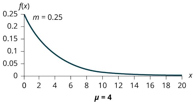
Figure A.5.1 — The exponential density for Sage's time with a customer, with decay parameter \(m = 0.25\) and mean 4 minutes. The maximum height on the \(y\)-axis is \(m\).
Answer: \(X \sim Exp(0.25)\), with \(f(x) = 0.25e^{-0.25x}\) for \(x \ge 0\), \(\mu = \sigma = 4\) minutes, and the declining curve shown in Figure A.5.1.
A.5.2 Finding Probabilities with the Cumulative Distribution Function
If \(X \sim Exp(m)\), the cumulative distribution function gives the area under the density curve to the left of \(x\):
$$ P(X < x) = 1 - e^{-mx}, \quad x \ge 0. $$The two companion forms follow immediately:
$$ P(X > x) = e^{-mx}, \qquad P(a < X < b) = e^{-ma} - e^{-mb}. $$The right-tail form is worth a second look, because it falls out of the left-tail one with no new work: \(P(X > x) = 1 - P(X < x) = 1 - \left(1 - e^{-mx}\right) = e^{-mx}\). That is as clean as probability formulas get — the chance of waiting longer than \(x\) is just \(e^{-mx}\).
Every exponential probability question reduces to areas to the left. "Less than" is one of them. "Greater than" is one minus one of them. "Between" is one minus the other. Learn the CDF and you have covered all three cases with a single formula.
Percentiles run the same machinery backwards. Instead of handing the formula an \(x\) and reading off an area, you hand it an area and solve for the \(x\). Because the CDF involves \(e\), undoing it takes a natural logarithm.
The value \(k\) with a given area to its left is
$$ k = \frac{\ln(1 - \text{AreaToTheLeft})}{-m}, $$where \(\ln\) is the natural log.
The one thing to be careful about with that formula is the phrase the problem uses. "The 30th percentile", "30% finish within", and "the value with 30% of the area to its left" all mean the same thing, and you feed 0.30 straight in. But "70% last at least this long" is describing the area to the RIGHT, so the area to the left is \(1 - 0.70 = 0.30\) and that is the number the formula wants. Sketching the curve and shading the region the sentence describes before you compute anything is the cheapest way to catch this, because a percentile computed from the wrong tail still comes out as a perfectly plausible-looking number. The next exercise asks for a probability and a median, so you will use both directions of the machinery.
Definition A.5.2 - The CDF value is the area collected so far: the boundary sweeps right and the readout climbs toward 1.
Mateo Delgado and his husband fly home for the holidays every year. The number of days ahead travelers like him purchase their airline tickets can be modeled by an exponential distribution with the average amount of time equal to 15 days. Find the probability that he will purchase a ticket fewer than ten days in advance. How many days do half of all travelers wait?
Solution
Let \(X\) = the number of days ahead a traveler purchases a ticket.
Step 1 — Decay parameter. \(\mu = 15\), so \(m = \frac{1}{15} \approx 0.0667\) and \(X \sim Exp\left(\frac{1}{15}\right)\).
Step 2 — Fewer than ten days. Use the CDF:
$$ P(x < 10) = 1 - e^{-\frac{10}{15}} = 1 - e^{-0.6667} \approx 0.4866 $$Step 3 — The median wait. Set the area to the left equal to 0.50 and use the percentile formula:
$$ k = \frac{\ln(1 - 0.50)}{-\frac{1}{15}} = \frac{\ln(0.50)}{-0.0667} \approx 10.40 \text{ days} $$Answer: About 0.4866, or roughly a 49% chance he buys fewer than ten days out; half of all travelers wait about 10.4 days.
Have each class member count the change they have in their pocket or purse. Your instructor will record the amounts in dollars and cents. Construct a histogram of the data taken by the class. Use five intervals. Draw a smooth curve through the bars. The graph should look approximately exponential. Then calculate the mean.
Let \(X\) = the amount of money a student in your class has in their pocket or purse.
The distribution for \(X\) is approximately exponential with mean \(\mu =\) ____ and \(m =\) ____. The standard deviation \(\sigma =\) ____.
Draw the appropriate exponential graph. You should label the \(x\)- and \(y\)-axes, the decay rate, and the mean. Shade the area that represents the probability that one student has less than $0.40 in their pocket or purse — that is, shade \(P(x < 0.40)\).
Build the class histogram without graph paper
The exercise wants a histogram of everyone's pocket change and then the mean of that same data, and rāSHio does both. Paste the amounts your instructor records into File → Delimited List… — it takes commas, semicolons, tabs, or one value per line, so the figures can go in exactly as they were read out. Then choose Graph → Histogram and set five intervals to match the exercise, and switch to Stats → Summary Statistics for the mean. Taking \(m = 1/\bar{x}\) fills in the decay parameter the exercise asks for, and the standard deviation the panel reports should land close to the mean — that near-equality is the exponential's fingerprint.
Figure A.5.2 — The rāSHio Summary Statistics panel: Stats → Summary Statistics. One panel for the mean, median, standard deviation and quartiles. The walkthrough uses its own demonstration numbers, not this exercise's.
The postal-clerk problem used minutes, but nothing in the formulas cares what the units are. The next example runs the same three moves — right tail, percentile, and a between-probability — on a part whose lifetime is measured in years. Watch how little changes: you still start by turning the mean into \(m\), you still reach for \(1 - e^{-mx}\) when the question says "less than", and you still take a natural log when the question hands you an area and asks for a time. The one genuinely new idea is part b, which asks about several parts used one after another. That is a question about a total, not about a probability, and it is answered by adding averages rather than by any exponential formula at all.
Using the information in Example A.5.1, where \(X \sim Exp(0.25)\):
a. Find the probability that Sage spends four to five minutes with a randomly selected customer.
b. Half of all customers are finished within how long? (Find the 50th percentile.)
c. Which is larger, the mean or the median?
Solution
Part a — Find \(P(4 < x < 5)\).
The cumulative distribution function gives the area to the left, so compute both left-hand areas and subtract:
$$ P(x < 5) = 1 - e^{(-0.25)(5)} = 0.7135 \quad \text{and} \quad P(x < 4) = 1 - e^{(-0.25)(4)} = 0.6321 $$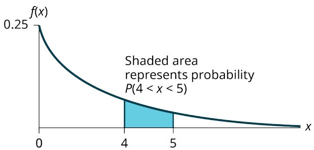
Figure A.5.3 — The shaded strip between \(x = 4\) and \(x = 5\) under the exponential density with \(m = 0.25\).
$$ P(4 < x < 5) = P(x < 5) - P(x < 4) = 0.7135 - 0.6321 = 0.0814 $$On a TI-83/83+/84/84+: on the home screen, enter (1 - e^(-0.25*5)) - (1 - e^(-0.25*4)), or the shorter equivalent e^(-0.25*4) - e^(-0.25*5).
The probability that Sage spends four to five minutes with a randomly selected customer is 0.0814.
Part b — Find the 50th percentile.
We want the value \(k\) with half the area to its left, so \(P(x < k) = 0.50\).
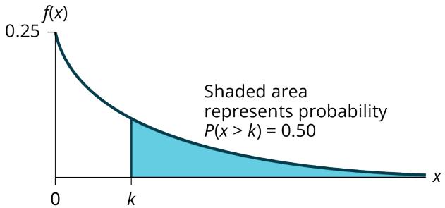
Figure A.5.4 — The 50th percentile \(k\) splits the area under the curve in half.
Set the CDF equal to 0.50 and solve:
$$ 0.50 = 1 - e^{-0.25k} \quad \Longrightarrow \quad e^{-0.25k} = 1 - 0.50 = 0.5 $$Take natural logs of both sides: \(\ln\left(e^{-0.25k}\right) = \ln(0.50)\), so \(-0.25k = \ln(0.50)\), and
$$ k = \frac{\ln(0.50)}{-0.25} = 2.8 \text{ minutes}. $$That is the percentile formula in action, with the area to the left equal to 0.50.
On a TI-83/83+/84/84+: on the home screen, enter ln(1 - 0.50)/-0.25. Press the (-) key for the negative sign.
Half of Sage's customers are finished within 2.8 minutes.
Part c — Compare the mean and the median.
From part b, the median (the 50th percentile) is 2.8 minutes. The theoretical mean is 4 minutes. The mean is larger.
Answer: (a) 0.0814; (b) 2.8 minutes; (c) the mean.
Jordan Okonkwo runs every morning before class. On average, a pair of their running shoes can last 18 months if used every day, and the length of time running shoes last is exponentially distributed. What is the probability that a pair of running shoes last more than 15 months? On average, how long would six pairs of running shoes last if they are used one after the other? Eighty percent of running shoes last at most how long if used every day?
Solution
Let \(X\) = the length of time, in months, a pair of their running shoes lasts.
Step 1 — Decay parameter. \(\mu = 18\), so \(m = \frac{1}{18} \approx 0.0556\) and \(X \sim Exp\left(\frac{1}{18}\right)\).
Step 2 — More than 15 months. Use the right-tail form:
$$ P(x > 15) = e^{-\frac{15}{18}} = e^{-0.8333} \approx 0.4346 $$Step 3 — Six pairs used one after another. Averages add:
$$ (6)(18) = 108 \text{ months} \ (= 9 \text{ years}) $$Step 4 — The 80th percentile.
$$ k = \frac{\ln(1 - 0.80)}{-\frac{1}{18}} = \frac{\ln(0.20)}{-0.0556} \approx 28.97 \text{ months} $$Answer: About 0.4346; 108 months on average for six pairs; 80% of pairs last at most about 29 months.
Lin Zhao and her wife run a computer repair shop. On the average, a certain part she replaces lasts ten years. The length of time the computer part lasts is exponentially distributed.
a. What is the probability that one of her computer parts lasts more than 7 years?
b. On the average, how long would five computer parts last if they are used one after another?
c. Eighty percent of computer parts last at most how long?
d. What is the probability that a computer part lasts between nine and 11 years?
Solution
Setup. Let \(x\) = the amount of time, in years, one of her computer parts lasts. Since \(\mu = 10\),
$$ m = \frac{1}{\mu} = \frac{1}{10} = 0.1, $$so \(X \sim Exp(0.1)\).
Part a — Find \(P(x > 7)\).
Use the right-tail form. Since \(P(X < x) = 1 - e^{-mx}\), we get \(P(X > x) = 1 - \left(1 - e^{-mx}\right) = e^{-mx}\), so
$$ P(x > 7) = e^{(-0.1)(7)} = 0.4966. $$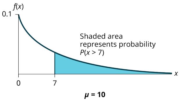
Figure A.5.5 — The shaded right tail beyond \(x = 7\) for an exponential distribution with \(m = 0.1\).
On a TI-83/83+/84/84+: on the home screen, enter e^(-.1*7).
The probability that a computer part lasts more than seven years is 0.4966.
Part b — Five parts used one after another.
This one needs no exponential formula. On average, one computer part lasts ten years, so five parts used one right after the other would last, on average,
$$ (5)(10) = 50 \text{ years}. $$Part c — Find the 80th percentile.
Let \(k\) = the 80th percentile, the lifetime with 80% of the area to its left.
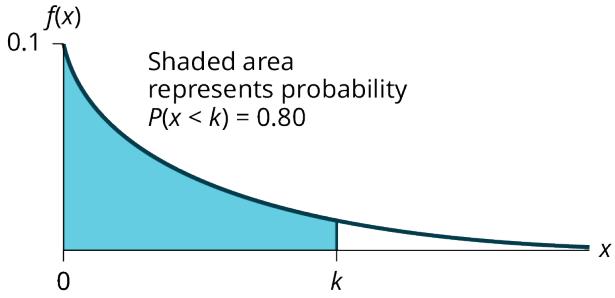
Figure A.5.6 — The 80th percentile \(k\), with 80% of the area to its left.
$$ k = \frac{\ln(1 - 0.80)}{-0.1} = 16.1 \text{ years} $$On a TI-83/83+/84/84+: on the home screen, enter ln(1-0.80)/-0.1.
Eighty percent of the computer parts last at most 16.1 years.
Part d — Find \(P(9 < x < 11)\).
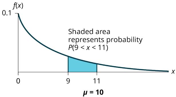
Figure A.5.7 — The shaded strip between \(x = 9\) and \(x = 11\).
$$ P(9 < x < 11) = P(x < 11) - P(x < 9) = \left(1 - e^{(-0.1)(11)}\right) - \left(1 - e^{(-0.1)(9)}\right) = 0.6671 - 0.5934 = 0.0737 $$On a TI-83/83+/84/84+: on the home screen, enter e^(-0.1*9) - e^(-0.1*11).
The probability that a computer part lasts between nine and 11 years is 0.0737.
Answer: (a) 0.4966; (b) 50 years; (c) 16.1 years; (d) 0.0737.
Daniel Whitfield and his husband are house-hunting outside of town. Suppose that the distance, in miles, that people are willing to commute to work is an exponential random variable with a decay parameter \(\frac{1}{20}\). Let \(X\) = the distance people are willing to commute in miles. What is \(m\), \(\mu\), and \(\sigma\)? What is the probability that a person is willing to commute more than 25 miles?
Solution
Step 1 — The three parameters.
- \(m = \frac{1}{20} = 0.05\)
- \(\mu = \frac{1}{m} = 20\) miles
- \(\sigma = \mu = 20\) miles
Step 2 — More than 25 miles.
$$ P(x > 25) = e^{-(0.05)(25)} = e^{-1.25} \approx 0.2865 $$Answer: \(m = 0.05\), \(\mu = \sigma = 20\) miles, and \(P(x > 25) \approx 0.2865\).
Suppose that the length of a phone call, in minutes, is an exponential random variable with decay parameter \(\frac{1}{12}\). If another person arrives at a public telephone just before you, find the probability that you will have to wait more than five minutes. Let \(X\) = the length of a phone call, in minutes.
What are \(m\), \(\mu\), and \(\sigma\)? The probability that you must wait more than five minutes is ____.
Solution
Step 1 — Read off the three parameters. The decay parameter is given directly:
- \(m = \frac{1}{12}\)
- \(\mu = \frac{1}{m} = 12\)
- \(\sigma = \mu = 12\)
Step 2 — Find the right-tail probability.
$$ P(x > 5) = e^{-\frac{5}{12}} = 0.6592 $$Answer: \(m = \frac{1}{12}\), \(\mu = 12\), \(\sigma = 12\), and \(P(x > 5) = 0.6592\).
A.5.3 Waiting Time Between Events
So far the exponential variable has been the lifetime of a single thing: one phone call, one computer part, one visit to a postal clerk. The distribution does its most useful work in a slightly different setting — as the gap between events in a stream of arrivals. Customers walk into a store, calls hit a switchboard, cars pass a point on a highway. If the events arrive at a steady average rate and do not coordinate with each other, the time you wait between two of them is exponential.
If 30 customers arrive per hour, one arrives every two minutes on average. The rate counts events per unit of time; the mean gap measures time per event. Flip one over and you have the other, which is why turning a stated rate into \(\mu\) is almost always the first move.
The catch is units. A problem will hand you a rate in customers per hour and then ask a question in minutes, or hand you calls per minute and ask about an eight-minute stretch. Before you touch a formula, convert the rate into the mean gap in whatever unit the question is written in, then take the reciprocal of that mean to get \(m\). Skipping this conversion is the single most common way these problems go wrong, and the mistake is invisible afterwards because the arithmetic still produces a perfectly reasonable-looking probability. There is a second habit worth building here too: these problems usually mix a waiting-time question with a plain averages question. "How long until the next car" needs the exponential formulas; "how long until seven more cars pass" needs nothing but multiplication, because averages add. Sort each part into one bucket or the other before you start, and half the work disappears.
Claire Bennett is waiting with her wife to pull out onto a certain stretch of highway, where cars pass at an average rate of five cars per minute. Assume that the duration of time between successive cars follows the exponential distribution.
a. On average, how many seconds elapse between two successive cars?
b. After a car passes by, how long on average will it take for another seven cars to pass by?
c. Find the probability that after a car passes by, the next car will pass within the next 20 seconds.
d. Find the probability that after a car passes by, the next car will not pass for at least another 15 seconds.
Solution
Part a — The average gap. Five cars per minute means one car every \(\frac{60}{5} = 12\) seconds on average.
Part b — Seven cars. \((7)(12) = 84\) seconds, or 1.4 minutes.
Part c — Within 20 seconds. Working in seconds, \(\mu = 12\), so \(m = \frac{1}{12}\) and \(X \sim Exp\left(\frac{1}{12}\right)\).
$$ P(X < 20) = 1 - e^{-\frac{20}{12}} = 1 - e^{-1.6667} \approx 0.8111 $$Part d — At least 15 seconds.
$$ P(X > 15) = e^{-\frac{15}{12}} = e^{-1.25} \approx 0.2865 $$Answer: (a) 12 seconds; (b) 84 seconds; (c) about 0.8111; (d) about 0.2865.
The time spent waiting between events is often modeled using the exponential distribution. Suppose that an average of 30 customers per hour arrive at a store and the time between arrivals is exponentially distributed.
a. On average, how many minutes elapse between two successive arrivals?
b. When the store first opens, how long on average does it take for three customers to arrive?
c. After a customer arrives, find the probability that it takes less than one minute for the next customer to arrive.
d. After a customer arrives, find the probability that it takes more than five minutes for the next customer to arrive.
e. Seventy percent of the customers arrive within how many minutes of the previous customer?
f. Is an exponential distribution reasonable for this situation?
Solution
Part a — The average gap. Since we expect 30 customers to arrive per hour (60 minutes), we expect on average one customer to arrive every two minutes.
Part b — Three customers. Since one customer arrives every two minutes on average, it will take six minutes on average for three customers to arrive.
Part c — Find \(P(X < 1)\).
Let \(X\) = the time between arrivals, in minutes. By part a, \(\mu = 2\), so \(m = \frac{1}{2} = 0.5\) and \(X \sim Exp(0.5)\).
The cumulative distribution function is \(P(X < x) = 1 - e^{(-0.5)(x)}\), so
$$ P(X < 1) = 1 - e^{(-0.5)(1)} \approx 0.3935. $$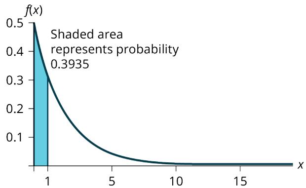
Figure A.5.8 — The shaded area to the left of \(x = 1\) for the time between customer arrivals.
On a TI-83/83+/84/84+: enter 1 - e^(-0.5), which returns 0.3935.
Part d — Find \(P(X > 5)\).
$$ P(X > 5) = 1 - P(X < 5) = 1 - \left(1 - e^{(-0.50)(5)}\right) = e^{-2.5} \approx 0.0821 $$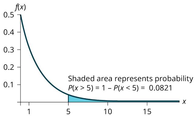
Figure A.5.9 — The shaded right tail beyond \(x = 5\) for the time between customer arrivals.
On a TI-83/83+/84/84+: enter 1 - (1 - e^((-0.50)(5))), or the shorter e^(-5*0.5).
Part e — Find the 70th percentile.
We want to solve \(0.70 = P(X < x)\) for \(x\). Substituting into the cumulative distribution function gives \(0.70 = 1 - e^{-0.5x}\), so \(e^{-0.5x} = 0.30\). Converting to logarithmic form gives \(-0.5x = \ln(0.30)\), or
$$ x = \frac{\ln(0.30)}{-0.5} \approx 2.41 \text{ minutes}. $$This is the percentile formula with the area to the left equal to 0.70:
$$ k = \frac{\ln(1 - 0.70)}{-0.5} \approx 2.41 \text{ minutes} $$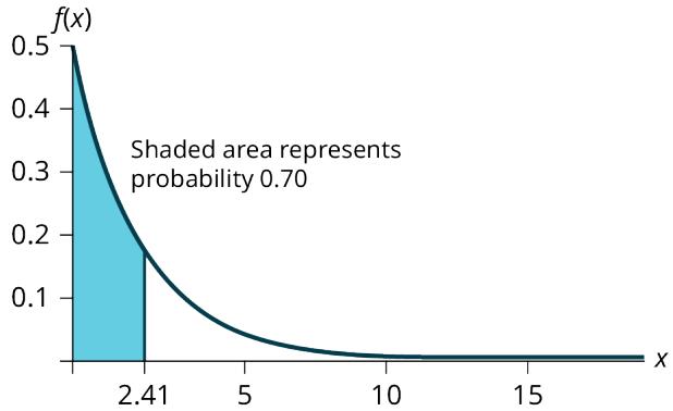
Figure A.5.10 — The 70th percentile of the time between customer arrivals, at about 2.41 minutes.
Seventy percent of customers arrive within 2.41 minutes of the previous customer.
Part f — Is the model reasonable?
This model assumes that a single customer arrives at a time, which may not be reasonable since people might shop in groups, leading to several customers arriving at the same time. It also assumes that the flow of customers does not change throughout the day, which is not valid if some times of the day are busier than others.
Answer: (a) 2 minutes; (b) 6 minutes; (c) 0.3935; (d) 0.0821; (e) 2.41 minutes; (f) no — group arrivals and time-of-day variation both break the model's assumptions.
A.5.4 Memorylessness of the Exponential Distribution
An exponential random variable \(X\) is memoryless: for all \(r \ge 0\) and \(t \ge 0\),
$$ P(X > r + t \mid X > r) = P(X > t). $$In words, the probability of waiting at least \(t\) more units of time is the same no matter how long \(r\) you have already waited.
This is where the exponential distribution stops behaving the way intuition expects. In Example A.5.5 the time between customers was exponentially distributed with a mean of two minutes, \(X \sim Exp(0.5)\). Suppose five minutes have gone by since the last customer arrived. Since an unusually long stretch has now passed, it feels like a customer is overdue — surely one is more likely to show up in the next minute than usual. The definition above says otherwise: the additional time spent waiting does not depend on how much time has already elapsed.
Take the store again. If five minutes have elapsed since the last customer arrived, the probability that more than one more minute passes before the next arrival uses \(r = 5\) and \(t = 1\):
$$ P(X > 5 + 1 \mid X > 5) = P(X > 1) = e^{(-0.5)(1)} \approx 0.6065. $$That is exactly the same probability as waiting more than one minute starting fresh, right after an arrival. The five minutes bought you nothing.
The exponential distribution is often used to model the longevity of an electrical or mechanical device, and there the memoryless property has a blunt physical meaning. In Example A.5.3 the lifetime of a computer part was exponential with a mean of ten years, \(X \sim Exp(0.1)\). Memorylessness says that knowing what has happened in the past has no effect on future probabilities: an old part is no more likely to break down at any particular time than a brand new one. The part stays as good as new until it suddenly breaks. If the part has already lasted ten years, the probability it lasts another seven is
$$ P(X > 17 \mid X > 10) = P(X > 7) = 0.4966, $$the same number we computed in Example A.5.3 for a fresh part.
Real machinery wears out — brake pads and batteries get likelier to fail as they age, so an exponential model would understate the risk on an old one. Memorylessness fits sudden, random failures and arrival streams, not gradual wear.
In practice, memorylessness is what lets you throw away the hardest-looking part of a conditional question. Whenever a problem says "given that it has already lasted \(r\)", cross that clause out and answer the plain question about the remaining time \(t\) — the two are the same number. The only work left is deciding what \(t\) actually is, and that is where these problems trip people up. A bulb that has lasted 12 years and is asked to reach a total of 19 has \(t = 7\), not 19; a customer four minutes in who needs three more minutes has \(t = 3\), not 7. Read the sentence for whether the second number is a total or an additional amount before you compute anything, and if it helps, write the two times on a number line and mark the gap between them — that gap is \(t\). Once you have it, the problem is an ordinary right-tail calculation: \(P(X > t) = e^{-mt}\), with the same \(m\) you would have used had nothing happened yet. Nothing about the conditional wording changes the formula; it only changes which number you feed it. The next exercise gives you a bulb that has already outlived its average, so the temptation to treat it as "due to fail" is exactly the instinct this section is training you out of.
Definition A.5.3 - Five minutes already waited buys nothing: the conditional curve is the same curve, so the same tail is shaded in the same place.
Riley Carter has never changed the bulb in their kitchen. Suppose that the longevity of a light bulb is exponential with a mean lifetime of eight years. If their bulb has already lasted 12 years, find the probability that it will last a total of over 19 years.
Solution
Let \(X\) = the lifetime of their light bulb, in years. \(\mu = 8\), so \(m = \frac{1}{8} = 0.125\) and \(X \sim Exp(0.125)\).
Step 1 — Translate the question. "Already lasted 12 years, lasts a total of over 19" is the conditional probability \(P(X > 19 \mid X > 12)\).
Step 2 — Apply memorylessness. With \(r = 12\) and \(t = 7\),
$$ P(X > 19 \mid X > 12) = P(X > 7). $$Step 3 — Compute.
$$ P(X > 7) = e^{-\frac{7}{8}} = e^{-0.875} \approx 0.4169 $$Answer: About 0.4169. The 12 years already logged make no difference.
Refer to Example A.5.1, where the time Sage spends with a customer has an exponential distribution with a mean of four minutes. Suppose a customer has already been at their window for four minutes. What is the probability that the customer will spend at least an additional three minutes with them?
Solution
Step 1 — Set up the distribution. The decay parameter of \(X\) is \(m = \frac{1}{4} = 0.25\), so \(X \sim Exp(0.25)\), and the cumulative distribution function is \(P(X < x) = 1 - e^{-0.25x}\).
Step 2 — Recognize the conditional question. We want \(P(X > 7 \mid X > 4)\). The memoryless property says
$$ P(X > 7 \mid X > 4) = P(X > 3), $$so the four minutes already spent drop out entirely, and we just need the probability that a customer spends more than three minutes with Sage.
Step 3 — Compute the right tail.
$$ P(X > 3) = 1 - P(X < 3) = 1 - \left(1 - e^{-0.25 \cdot 3}\right) = e^{-0.75} \approx 0.4724 $$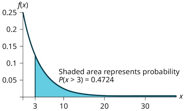
Figure A.5.11 — The shaded right tail beyond \(x = 3\), which by memorylessness answers the conditional question.
On a TI-83/83+/84/84+: enter 1 - (1 - e^(-0.25*3)), or the shorter e^(-0.25*3).
Answer: About 0.4724.
A.5.5 The Poisson and the Exponential: Two Views of One Process
There is a tight relationship between the exponential distribution and the Poisson distribution you met in the chapter on discrete random variables. They describe the same stream of events from two different angles: the exponential measures the time between events, and the Poisson counts the number of events in a fixed stretch.
Suppose the time that elapses between two successive events follows the exponential distribution with a mean of \(\mu\) units of time, and assume those times are independent — the gap between two events is not affected by the gaps that came before. If those assumptions hold, then the number of events per unit time follows a Poisson distribution with mean \(\lambda = \frac{1}{\mu}\). Recall that if \(X\) has the Poisson distribution with mean \(\lambda\), then
$$ P(X = k) = \frac{\lambda^k e^{-\lambda}}{k!}, \qquad k! = k \cdot (k-1) \cdot (k-2) \cdot (k-3) \cdots 3 \cdot 2 \cdot 1. $$The relationship runs both directions. If the number of events per unit time follows a Poisson distribution, then the amount of time between events follows the exponential distribution.
Read Poisson probabilities off a panel
You do not need a graphing calculator for the counting half of this section. In rāSHio, choose Distributions → Poisson and set the mean to the \(\lambda\) the problem gives you — the panel calls it \(\lambda\), which is the same number this book writes as the average count for the interval. Pick Exact for \(P(X = k)\), Left for \(P(X \le k)\), or Right for the "more than" questions, then enter \(k\). A mean of 4 with Exact at \(k = 5\) returns the 0.1563 worked out below, and a mean of 32 with Right at \(k = 40\) returns the 0.0707. The panel draws the bars as well as reporting the number, so you can see which counts actually carry the probability.
Figure A.5.12 — The rāSHio Poisson panel: Distributions → Poisson. Set the mean, pick a region, read the probability. The walkthrough uses its own demonstration numbers, not this section's.
In a small city, the number of automobile accidents occur with a Poisson distribution at an average of three per week.
a. Calculate the probability that there are at most 2 accidents occur in any given week.
b. What is the probability that there is at least two weeks between any 2 accidents?
Solution
Part a — At most 2 accidents in a week.
Let \(X\) = the number of accidents in a week, so \(X \sim Poisson(3)\).
$$ P(X \le 2) = \frac{3^0 e^{-3}}{0!} + \frac{3^1 e^{-3}}{1!} + \frac{3^2 e^{-3}}{2!} = e^{-3}(1 + 3 + 4.5) \approx 0.4232 $$On a calculator, poissoncdf(3, 2) = 0.4232.
Part b — At least two weeks between accidents.
Switch to the waiting-time view. If accidents average three per week, the mean time between accidents is \(\mu = \frac{1}{3}\) week, so \(m = 3\) and \(T \sim Exp(3)\) with \(T\) measured in weeks.
$$ P(T > 2) = e^{-(3)(2)} = e^{-6} \approx 0.0025 $$Answer: (a) about 0.4232; (b) about 0.0025 — a two-week gap between accidents is very unlikely at this rate.
At a police station in a large city, calls come in at an average rate of four calls per minute. Assume that the time that elapses from one call to the next has the exponential distribution. Take note that we are concerned only with the rate at which calls come in, and we are ignoring the time spent on the phone. We must also assume that the times spent between calls are independent — a particularly long delay between two calls does not mean there will be a shorter waiting period for the next call. We may then deduce that the total number of calls received during a time period has the Poisson distribution.
a. Find the average time between two successive calls.
b. Find the probability that after a call is received, the next call occurs in less than ten seconds.
c. Find the probability that exactly five calls occur within a minute.
d. Find the probability that less than five calls occur within a minute.
e. Find the probability that more than 40 calls occur in an eight-minute period.
Solution
Part a — The average gap. On average four calls occur per minute, so \(\frac{15}{60} = 0.25\) minutes — that is, 15 seconds — occur between successive calls on average.
Part b — Less than ten seconds.
Let \(T\) = time elapsed between calls. From part a, \(\mu = 0.25\), so \(m = \frac{1}{0.25} = 4\) and \(T \sim Exp(4)\). The cumulative distribution function is \(P(T < t) = 1 - e^{-4t}\).
Ten seconds is \(\frac{1}{6}\) of a minute, so
$$ P\left(T < \frac{1}{6}\right) = 1 - e^{(-4)\left(\frac{1}{6}\right)} \approx 0.4866. $$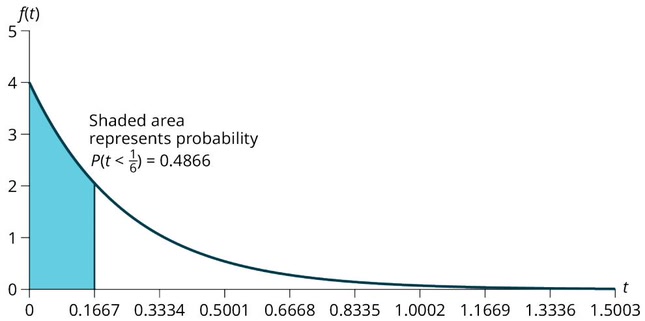
Figure A.5.13 — The shaded area to the left of \(t = \frac{1}{6}\) minute for the time between police calls.
Part c — Exactly five calls in a minute.
Now switch to the counting view. Let \(X\) = the number of calls per minute. As stated above, the number of calls per minute has a Poisson distribution with a mean of four calls per minute, so \(X \sim Poisson(4)\) and
$$ P(X = 5) = \frac{4^5 e^{-4}}{5!} \approx 0.1563, \qquad 5! = (5)(4)(3)(2)(1). $$On a TI-83/83+/84/84+: poissonpdf(4, 5) = 0.1563.
Part d — Less than five calls in a minute.
Keep in mind that \(X\) must be a whole number, so \(P(X < 5) = P(X \le 4)\). We could take \(P(X = 0) + P(X = 1) + P(X = 2) + P(X = 3) + P(X = 4)\); using technology,
$$ P(X \le 4) = 0.6288. $$On a TI-83/83+/84/84+: poissoncdf(4, 4) = 0.6288.
Part e — More than 40 calls in eight minutes.
Let \(Y\) = the number of calls that occur during an eight-minute period. Since there is an average of four calls per minute, there is an average of \((8)(4) = 32\) calls during each eight-minute period, so \(Y \sim Poisson(32)\) and
$$ P(Y > 40) = 1 - P(Y \le 40) = 1 - 0.9294 = 0.0707. $$On a TI-83/83+/84/84+: 1 - poissoncdf(32, 40) = 0.0707.
Answer: (a) 15 seconds; (b) 0.4866; (c) 0.1563; (d) 0.6288; (e) 0.0707.
Problem Set A.5
Use the following information to answer the next ten exercises. Hector Reyes is a customer service representative, and he must spend different amounts of time with each customer to resolve various concerns. The amount of time he spends with each customer can be modeled by the following distribution: \(X \sim Exp(0.2)\).
Problem 1. What type of distribution is this?
Solution
Step 1 — Read the notation: The problem states \(X \sim Exp(0.2)\), and \(Exp\) is the notation for the exponential distribution with decay parameter \(m\).
Answer: This is an exponential distribution, with decay parameter \(m = 0.2\).
Problem 2. Are outcomes equally likely in this distribution? Why or why not?
Solution
Step 1 — Recall the shape: The exponential density \(f(x) = 0.2e^{-0.2x}\) starts at its highest point when \(x = 0\) and declines from there. Short times sit under the tall part of the curve; long times sit under the thin tail.
Answer: No, outcomes are not equally likely. In this distribution, more people require a little bit of time, and fewer people require a lot of time, so it is more likely that someone will require less time.
Problem 3. What is \(m\)? What does it represent?
Solution
Step 1 — Read it off the notation: In \(X \sim Exp(m)\), the number in parentheses is \(m\), so \(m = 0.2\).
Step 2 — Say what it means: \(m\) is the decay parameter. It is the reciprocal of the mean, \(m = \frac{1}{\mu}\), so it converts an average waiting time into a rate. It is also the height of the density curve at \(x = 0\), which is why a larger \(m\) makes the curve start higher and fall away faster.
Answer: \(m = 0.2\), the decay parameter — the reciprocal of the mean, and the height of the curve at \(x = 0\).
Problem 4. What is the mean?
Solution
Step 1 — Invert the decay parameter:
$$ \mu = \frac{1}{m} = \frac{1}{0.2} = 5 $$Answer: Five minutes.
Problem 5. What is the standard deviation?
Solution
Step 1 — Use the exponential's defining property: For every exponential distribution the standard deviation equals the mean, \(\sigma = \mu\).
Answer: Five minutes.
Problem 6. State the probability density function.
Solution
Step 1 — Substitute \(m = 0.2\) into \(f(x) = me^{-mx}\):
$$ f(x) = 0.2e^{-0.2x}, \quad x \ge 0 $$Answer: \(f(x) = 0.2e^{-0.2x}\) for \(x \ge 0\).
Problem 7. Graph the distribution.
Solution
Step 1 — Find the starting height: At \(x = 0\), \(f(0) = 0.2e^{0} = 0.2\), so the curve meets the \(y\)-axis at 0.2 — the value of \(m\).
Step 2 — Plot a few more heights to fix the shape: \(f(5) = 0.2e^{-1} \approx 0.074\), \(f(10) = 0.2e^{-2} \approx 0.027\), \(f(20) = 0.2e^{-4} \approx 0.004\).
Step 3 — Draw it: Label the horizontal axis \(x\) (time in minutes) and the vertical axis \(f(x)\). Start the curve at \((0, 0.2)\) and let it fall smoothly to the right, flattening out toward the \(x\)-axis without ever touching it. Mark the mean \(\mu = 5\) on the horizontal axis.
Answer: A declining curve starting at height 0.2 on the \(y\)-axis and approaching the \(x\)-axis as \(x\) grows, with \(\mu = 5\) marked.
Problem 8. Find \(P(2 < x < 10)\).
Solution
Step 1 — Use the between-form: For an exponential distribution, \(P(a < X < b) = e^{-ma} - e^{-mb}\).
Step 2 — Substitute \(m = 0.2\), \(a = 2\), \(b = 10\):
$$ P(2 < x < 10) = e^{(-0.2)(2)} - e^{(-0.2)(10)} = e^{-0.4} - e^{-2} = 0.6703 - 0.1353 $$Answer: 0.5350.
Problem 9. Find \(P(x > 6)\).
Solution
Step 1 — Use the right-tail form: \(P(X > x) = e^{-mx}\).
Step 2 — Substitute:
$$ P(x > 6) = e^{(-0.2)(6)} = e^{-1.2} $$Answer: 0.3012.
Problem 10. Find the 70th percentile.
Solution
Step 1 — Use the percentile formula: \(k = \dfrac{\ln(1 - \text{AreaToTheLeft})}{-m}\), with area to the left 0.70.
Step 2 — Substitute:
$$ k = \frac{\ln(1 - 0.70)}{-0.2} = \frac{\ln(0.30)}{-0.2} = \frac{-1.2040}{-0.2} $$Answer: \(k = 6.02\) minutes. Seventy percent of customers are handled within about 6 minutes.
Use the following information to answer the next eight exercises. A distribution is given as \(X \sim Exp(0.75)\).
Problem 11. What is \(m\)?
Solution
Step 1 — Read the notation: In \(X \sim Exp(m)\), the number in parentheses is the decay parameter.
Answer: \(m = 0.75\).
Problem 12. What is the probability density function?
Solution
Step 1 — Substitute \(m = 0.75\) into \(f(x) = me^{-mx}\):
$$ f(x) = 0.75e^{-0.75x}, \quad x \ge 0 $$Answer: \(f(x) = 0.75e^{-0.75x}\) for \(x \ge 0\).
Problem 13. What is the cumulative distribution function?
Solution
Step 1 — Substitute \(m = 0.75\) into \(P(X < x) = 1 - e^{-mx}\):
$$ P(X < x) = 1 - e^{-0.75x}, \quad x \ge 0 $$Answer: \(P(X < x) = 1 - e^{-0.75x}\).
Problem 14. Draw the distribution.
Solution
Step 1 — Find the starting height: \(f(0) = 0.75e^{0} = 0.75\), so the curve begins at 0.75 on the \(y\)-axis.
Step 2 — Get a few more points: \(f(2) = 0.75e^{-1.5} \approx 0.17\), \(f(4) = 0.75e^{-3} \approx 0.037\), \(f(6) = 0.75e^{-4.5} \approx 0.008\).
Step 3 — Draw it: Label the horizontal axis \(x\) and the vertical axis \(f(x)\). Start at \((0, 0.75)\) and fall away steeply — because \(m\) is large here, the curve drops much faster than the \(m = 0.2\) curve in the earlier group and is essentially flat by \(x = 6\).
Answer: A steeply declining curve starting at 0.75 on the \(y\)-axis and hugging the \(x\)-axis past about \(x = 6\).
Problem 15. Find \(P(x < 4)\).
Solution
Step 1 — Use the cumulative distribution function:
$$ P(x < 4) = 1 - e^{(-0.75)(4)} = 1 - e^{-3} = 1 - 0.0498 $$Answer: 0.9502.
Problem 16. Find the 30th percentile.
Solution
Step 1 — Use the percentile formula with area to the left 0.30:
$$ k = \frac{\ln(1 - 0.30)}{-0.75} = \frac{\ln(0.70)}{-0.75} = \frac{-0.3567}{-0.75} $$Answer: \(k = 0.4756\).
Problem 17. Find the median.
Solution
Step 1 — The median is the 50th percentile: use the percentile formula with area to the left 0.50.
$$ k = \frac{\ln(1 - 0.50)}{-0.75} = \frac{\ln(0.50)}{-0.75} = \frac{-0.6931}{-0.75} $$Answer: The median is 0.9242.
Problem 18. Which is larger, the mean or the median?
Solution
Step 1 — Compute the mean: \(\mu = \frac{1}{m} = \frac{1}{0.75} \approx 1.33\).
Step 2 — Compare with the median from the previous problem: the median is 0.9242.
Step 3 — Explain why: The long right tail pulls the mean upward, while the median only has to split the area in half. For every exponential distribution the mean sits to the right of the median.
Answer: The mean is larger. The mean is \(\frac{1}{m} = \frac{1}{0.75} \approx 1.33\), which is greater than 0.9242.
Use the following information to answer the next eight exercises. Carbon-14 is a radioactive element with a half-life of about 5,730 years. Carbon-14 is said to decay exponentially. The decay rate is 0.000121. We start with one gram of carbon-14. We are interested in the time (years) it takes to decay carbon-14.
Problem 19. What is being measured here?
Solution
Step 1 — Identify the quantity of interest: The setup says we are interested in the time it takes carbon-14 to decay, and it gives that time in years.
Answer: The amount of time, in years, it takes for carbon-14 to decay.
Problem 20. Are the data discrete or continuous?
Solution
Step 1 — Ask whether the values are counted or measured: Time is measured, not counted, and can take any value in an interval.
Answer: Continuous.
Problem 21. In words, define the random variable \(X\).
Solution
Step 1 — Name the variable in words, with its units:
Answer: \(X\) = the time, in years, it takes for carbon-14 to decay.
Problem 22. What is the decay rate \(m\)?
Solution
Step 1 — Read it from the setup: The problem states the decay rate directly.
Answer: \(m = 0.000121\).
Problem 23. The distribution for \(X\) is ____.
Solution
Step 1 — Write the distribution notation with the given decay parameter:
Answer: \(X \sim Exp(0.000121)\).
Problem 24. Find the amount (percent of one gram) of carbon-14 lasting less than 5,730 years. This means, find \(P(x < 5{,}730)\).
a) Sketch the graph, and shade the area of interest.
b) Find the probability. \(P(x < 5{,}730) =\) ____
Solution
Part a — Sketch and shade. Draw the declining exponential curve with the horizontal axis labelled \(x\) (years) and the vertical axis labelled \(f(x)\). Mark 5,730 on the horizontal axis and shade the region under the curve from 0 to 5,730 — the area to the LEFT, because the question asks for "less than". Answers may vary in scale.
Part b — Compute the probability. Use the cumulative distribution function with \(m = 0.000121\):
$$ P(x < 5{,}730) = 1 - e^{(-0.000121)(5{,}730)} = 1 - e^{-0.6933} = 1 - 0.4999 $$Answer: \(P(x < 5{,}730) = 0.5001\). About half of one gram of carbon-14 decays within 5,730 years, which is exactly what "half-life of about 5,730 years" means.
Problem 25. Find the percentage of carbon-14 lasting longer than 10,000 years.
a) Sketch the graph, and shade the area of interest.
b) Find the probability. \(P(x > 10{,}000) =\) ____
Solution
Part a — Sketch and shade. Draw the same declining curve, mark 10,000 on the horizontal axis, and shade the region to the RIGHT of it — "longer than" is a right tail. Answers may vary in scale.
Part b — Compute the probability. Use the right-tail form \(P(X > x) = e^{-mx}\):
$$ P(x > 10{,}000) = e^{(-0.000121)(10{,}000)} = e^{-1.21} $$Answer: \(P(x > 10{,}000) = 0.2982\), so about 29.82% of the carbon-14 lasts longer than 10,000 years.
Problem 26. Thirty percent (30%) of carbon-14 will decay within how many years?
a) Sketch the graph, and shade the area of interest.
b) Find the value \(k\) such that \(P(x < k) = 0.30\).
Solution
Part a — Sketch and shade. Draw the declining curve, mark an unknown value \(k\) on the horizontal axis, and shade the region from 0 to \(k\) so that the shaded area is 30% of the total. Answers may vary in scale.
Part b — Solve for \(k\). Use the percentile formula with area to the left 0.30:
$$ k = \frac{\ln(1 - 0.30)}{-0.000121} = \frac{\ln(0.70)}{-0.000121} = \frac{-0.3567}{-0.000121} $$Answer: \(k = 2{,}947.73\) years. Thirty percent of the carbon-14 decays within about 2,948 years.
Problem 27. Suppose that the length of phone calls, measured in minutes, is known to have an exponential distribution with the average length of a call equal to eight minutes.
a) Define the random variable. \(X =\) ____.
b) Is \(X\) continuous or discrete?
c) \(X \sim\) ____
d) \(\mu =\) ____
e) \(\sigma =\) ____
f) Draw a graph of the probability distribution. Label the axes.
g) Find the probability that a phone call lasts less than nine minutes.
h) Find the probability that a phone call lasts more than nine minutes.
i) Find the probability that a phone call lasts between seven and nine minutes.
j) If 25 phone calls are made one after another, on average, what would you expect the total to be? Why?
Solution
Part a — Define the variable. \(X\) = the length of a phone call, in minutes.
Part b — Continuous or discrete? Continuous, because time is measured rather than counted.
Part c — The distribution. The mean is 8 minutes, so \(m = \frac{1}{8} = 0.125\) and \(X \sim Exp(0.125)\).
Part d — The mean. \(\mu = 8\) minutes.
Part e — The standard deviation. \(\sigma = \mu = 8\) minutes.
Part f — The graph. Label the horizontal axis \(x\) (minutes) and the vertical axis \(f(x)\). The curve starts at \(f(0) = m = 0.125\) and declines smoothly toward the \(x\)-axis.
Part g — Less than nine minutes.
$$ P(x < 9) = 1 - e^{(-0.125)(9)} = 1 - e^{-1.125} = 1 - 0.3247 = 0.6753 $$Part h — More than nine minutes. This is the complement of part g:
$$ P(x > 9) = e^{-1.125} = 0.3247 $$Part i — Between seven and nine minutes.
$$ P(7 < x < 9) = e^{(-0.125)(7)} - e^{(-0.125)(9)} = 0.4169 - 0.3247 = 0.0922 $$Part j — Twenty-five calls in a row. Averages add, so \((25)(8) = 200\) minutes. Each call averages eight minutes regardless of how the previous ones went, so 25 of them average 25 times as long.
Answer: (a) length of a call in minutes; (b) continuous; (c) \(X \sim Exp(0.125)\); (d) 8; (e) 8; (f) declining curve from 0.125; (g) 0.6753; (h) 0.3247; (i) 0.0922; (j) 200 minutes.
Problem 28. Suppose that the useful life of a particular car battery, measured in months, decays with parameter 0.025. We are interested in the life of the battery.
a) Define the random variable. \(X =\) ____.
b) Is \(X\) continuous or discrete?
c) \(X \sim\) ____
d) On average, how long would you expect one car battery to last?
e) On average, how long would you expect nine car batteries to last, if they are used one after another?
f) Find the probability that a car battery lasts more than 36 months.
g) Seventy percent of the batteries last at least how long?
Solution
Part a — Define the variable. \(X\) = the useful life of a particular car battery, measured in months.
Part b — Continuous or discrete? \(X\) is continuous.
Part c — The distribution. \(X \sim Exp(0.025)\).
Part d — One battery. \(\mu = \frac{1}{m} = \frac{1}{0.025} = 40\) months.
Part e — Nine batteries in a row. \((9)(40) = 360\) months.
Part f — More than 36 months.
$$ P(x > 36) = e^{(-0.025)(36)} = e^{-0.9} = 0.4066 $$Part g — Seventy percent last at least how long? "At least" means 70% of the area is to the RIGHT, so 30% is to the left. Use the percentile formula with area to the left 0.30:
$$ k = \frac{\ln(1 - 0.30)}{-0.025} = \frac{\ln(0.70)}{-0.025} = 14.27 \text{ months} $$Answer: (a) useful life in months; (b) continuous; (c) \(X \sim Exp(0.025)\); (d) 40 months; (e) 360 months; (f) 0.4066; (g) 14.27 months.
Problem 29. At one point in time, the percent of persons (ages five and older) in each state who speak a language at home other than English is approximately exponentially distributed with a mean of 9.848. Suppose we randomly pick a state.
a) Define the random variable. \(X =\) ____.
b) Is \(X\) continuous or discrete?
c) \(X \sim\) ____
d) \(\mu =\) ____
e) \(\sigma =\) ____
f) Draw a graph of the probability distribution. Label the axes.
g) Find the probability that the percent is less than 12.
h) Find the probability that the percent is between eight and 14.
i) The percent of all individuals living in the United States who speak a language at home other than English is 13.8. Why is this number different from 9.848%? What would make this number higher than 9.848%?
Solution
Part a — Define the variable. \(X\) = the percent of persons (ages five and older) in a randomly picked state who speak a language at home other than English.
Part b — Continuous or discrete? Continuous — a percent can take any value in a range.
Part c — The distribution. \(\mu = 9.848\), so \(m = \frac{1}{9.848} \approx 0.1015\) and \(X \sim Exp(0.1015)\).
Part d — The mean. \(\mu = 9.848\).
Part e — The standard deviation. \(\sigma = \mu = 9.848\).
Part f — The graph. Label the horizontal axis \(x\) (percent) and the vertical axis \(f(x)\). The curve starts at \(f(0) = m \approx 0.1015\) and declines toward the \(x\)-axis.
Part g — Less than 12 percent.
$$ P(x < 12) = 1 - e^{-\frac{12}{9.848}} = 1 - e^{-1.2185} = 1 - 0.2957 = 0.7043 $$Part h — Between eight and 14 percent.
$$ P(8 < x < 14) = e^{-\frac{8}{9.848}} - e^{-\frac{14}{9.848}} = 0.4438 - 0.2413 = 0.2025 $$Part i — Why 13.8% differs from 9.848%. The 9.848 figure is the average of the fifty state percentages, so every state counts once no matter how many people live in it. The 13.8 figure is a single national percentage, which counts every person once. States with very large populations and high percentages — California, Texas, New York — pull the national number up while contributing only one value apiece to the state-by-state average. Anything that concentrates non-English speakers into the biggest states raises the national number relative to the state average.
Answer: (a) the state's percent; (b) continuous; (c) \(X \sim Exp(0.1015)\); (d) 9.848; (e) 9.848; (f) declining curve from about 0.1015; (g) 0.7043; (h) 0.2025; (i) the national figure weights people, the 9.848 average weights states equally.
Problem 30. The time (in years) after reaching age 60 that it takes an individual to retire is approximately exponentially distributed with a mean of about five years. Suppose we randomly pick one retired individual. We are interested in the time after age 60 to retirement.
a) Define the random variable. \(X =\) ____.
b) Is \(X\) continuous or discrete?
c) \(X \sim\) ____
d) \(\mu =\) ____
e) \(\sigma =\) ____
f) Draw a graph of the probability distribution. Label the axes.
g) Find the probability that the person retired after age 70.
h) Do more people retire before age 65 or after age 65?
i) In a room of 1,000 people over age 80, how many do you expect will NOT have retired yet?
Solution
Part a — Define the variable. \(X\) = the time (in years) after reaching age 60 that it takes an individual to retire.
Part b — Continuous or discrete? \(X\) is continuous.
Part c — The distribution. \(X \sim Exp\left(\frac{1}{5}\right)\).
Part d — The mean. \(\mu = 5\) years.
Part e — The standard deviation. \(\sigma = \mu = 5\) years.
Part f — The graph. A declining curve starting at \(f(0) = 0.2\), with the horizontal axis labelled "years after age 60". Answers may vary in scale.
Part g — Retired after age 70. Age 70 is ten years after 60, so we want \(P(x > 10)\):
$$ P(x > 10) = e^{(-0.2)(10)} = e^{-2} = 0.1353 $$Part h — Before or after 65? Age 65 is five years after 60, and
$$ P(x < 5) = 1 - e^{(-0.2)(5)} = 1 - e^{-1} = 0.6321, $$which is more than half. More people retire before age 65.
Part i — 1,000 people over age 80. Age 80 is twenty years after 60, so the fraction not yet retired is \(P(x > 20) = e^{-4} = 0.0183\), and \((1{,}000)(0.0183) = 18.3\).
Answer: (a) years after 60 to retirement; (b) continuous; (c) \(X \sim Exp\left(\frac{1}{5}\right)\); (d) five; (e) five; (f) answers may vary; (g) 0.1353; (h) before; (i) about 18.3 people.
Problem 31. The cost of all maintenance for a car during its first year is approximately exponentially distributed with a mean of $150.
a) Define the random variable. \(X =\) ____.
b) \(X \sim\) ____
c) \(\mu =\) ____
d) \(\sigma =\) ____
e) Draw a graph of the probability distribution. Label the axes.
f) Find the probability that a car required over $300 for maintenance during its first year.
Solution
Part a — Define the variable. \(X\) = the cost, in dollars, of all maintenance for a car during its first year.
Part b — The distribution. \(\mu = 150\), so \(m = \frac{1}{150} \approx 0.00667\) and \(X \sim Exp\left(\frac{1}{150}\right)\).
Part c — The mean. \(\mu = \$150\).
Part d — The standard deviation. \(\sigma = \mu = \$150\).
Part e — The graph. Label the horizontal axis \(x\) (dollars) and the vertical axis \(f(x)\). The curve starts at \(f(0) = \frac{1}{150} \approx 0.0067\) and declines toward the \(x\)-axis.
Part f — Over $300.
$$ P(x > 300) = e^{-\frac{300}{150}} = e^{-2} = 0.1353 $$Answer: (a) first-year maintenance cost in dollars; (b) \(X \sim Exp\left(\frac{1}{150}\right)\); (c) $150; (d) $150; (e) declining curve from about 0.0067; (f) 0.1353.
Use the following information to answer the next three exercises. The average lifetime of a certain new smartphone is three years. The manufacturer will replace any smartphone failing within two years of the date of purchase. The lifetime of these smartphones is known to follow an exponential distribution.
Problem 32. The decay rate is:
a) 0.3333
b) 0.5000
c) 2
d) 3
Solution
Step 1 — Turn the average lifetime into a decay rate: The mean is three years, and the decay rate is the reciprocal of the mean:
$$ m = \frac{1}{\mu} = \frac{1}{3} = 0.3333 $$Answer: a. 0.3333
Problem 33. What is the probability that a smartphone will fail within two years of the date of purchase?
a) 0.8647
b) 0.4866
c) 0.2212
d) 0.9997
Solution
Step 1 — Recognize the question: "Fail within two years" is a "less than" question, so use the cumulative distribution function with \(m = \frac{1}{3}\).
Step 2 — Compute:
$$ P(x < 2) = 1 - e^{-\frac{2}{3}} = 1 - 0.5134 = 0.4866 $$Answer: b. 0.4866
Problem 34. What is the median lifetime of these phones (in years)?
a) 0.1941
b) 1.3863
c) 2.0794
d) 5.5452
Solution
Step 1 — The median is the 50th percentile:
$$ k = \frac{\ln(1 - 0.50)}{-\frac{1}{3}} = \frac{\ln(0.50)}{-0.3333} = \frac{-0.6931}{-0.3333} = 2.0794 $$Step 2 — Sanity-check: the median should be below the three-year mean, and 2.0794 is.
Answer: c. 2.0794
Problem 35. Let \(X \sim Exp(0.1)\).
a) decay rate = ____
b) \(\mu =\) ____
c) Graph the probability distribution function.
d) On the graph, shade the area corresponding to \(P(x < 6)\) and find the probability.
e) Sketch a new graph, shade the area corresponding to \(P(3 < x < 6)\) and find the probability.
f) Sketch a new graph, shade the area corresponding to \(P(x < 7)\) and find the probability.
g) Sketch a new graph, shade the area corresponding to the 40th percentile and find the value.
h) Find the average value of \(x\).
Solution
Part a — The decay rate. It is the number in the notation: \(m = 0.1\).
Part b — The mean. \(\mu = \frac{1}{m} = \frac{1}{0.1} = 10\).
Part c — The graph. Label the horizontal axis \(x\) and the vertical axis \(f(x)\). The curve \(f(x) = 0.1e^{-0.1x}\) starts at \((0, 0.1)\) and declines toward the \(x\)-axis, still visibly above it out past \(x = 30\).
Part d — \(P(x < 6)\). Shade from 0 to 6.
$$ P(x < 6) = 1 - e^{(-0.1)(6)} = 1 - 0.5488 = 0.4512 $$Part e — \(P(3 < x < 6)\). Shade the strip between 3 and 6.
$$ P(3 < x < 6) = e^{-0.3} - e^{-0.6} = 0.7408 - 0.5488 = 0.1920 $$Part f — \(P(x < 7)\). Shade from 0 to 7.
$$ P(x < 7) = 1 - e^{-0.7} = 1 - 0.4966 = 0.5034 $$Part g — The 40th percentile. Shade from 0 to \(k\) so the shaded area is 40% of the total.
$$ k = \frac{\ln(1 - 0.40)}{-0.1} = \frac{\ln(0.60)}{-0.1} = 5.11 $$Part h — The average value of \(x\). Same as part b: \(\mu = 10\).
Answer: (a) 0.1; (b) 10; (c) declining curve from 0.1; (d) 0.4512; (e) 0.1920; (f) 0.5034; (g) 5.11; (h) 10.
Problem 36. Suppose that the longevity of a light bulb is exponential with a mean lifetime of eight years.
a) Find the probability that a light bulb lasts less than one year.
b) Find the probability that a light bulb lasts between six and ten years.
c) Seventy percent of all light bulbs last at least how long?
d) A company decides to offer a warranty to give refunds to light bulbs whose lifetime is among the lowest two percent of all bulbs. To the nearest month, what should be the cutoff lifetime for the warranty to take place?
e) If a light bulb has lasted seven years, what is the probability that it fails within the 8th year?
Solution
Setup. Let \(T\) = the lifetime of a light bulb, in years. The decay parameter is \(m = \frac{1}{8}\), so \(T \sim Exp\left(\frac{1}{8}\right)\) and the cumulative distribution function is \(P(T < t) = 1 - e^{-\frac{t}{8}}\).
Part a — Less than one year.
$$ P(T < 1) = 1 - e^{-\frac{1}{8}} \approx 0.1175 $$Part b — Between six and ten years.
$$ P(6 < t < 10) = \left(1 - e^{-\frac{10}{8}}\right) - \left(1 - e^{-\frac{6}{8}}\right) \approx 0.7135 - 0.5276 = 0.1859 $$Part c — Seventy percent last at least how long? Here 70% of the area is to the RIGHT, so \(P(T > t) = e^{-\frac{t}{8}} = 0.70\). Taking logs, \(-\frac{t}{8} = \ln(0.70)\), so
$$ t = -8\ln(0.70) \approx 2.85 \text{ years}. $$Equivalently, \(t = \frac{\ln(\text{area to the right})}{-m} = \frac{\ln(0.70)}{-\frac{1}{8}} \approx 2.85\) years.
Part d — The warranty cutoff (lowest two percent). Use the percentile formula with area to the left 0.02:
$$ k = \frac{\ln(1 - 0.02)}{-\frac{1}{8}} = \frac{\ln(0.98)}{-0.125} \approx 0.1616 \text{ years} $$Converting, \((0.1616)(12) \approx 1.94\) months, which rounds to 2 months.
Part e — Fails during the 8th year, given it has lasted seven. By the memoryless property, \(P(7 < T < 8 \mid T > 7) = P(T < 1) \approx 0.1175\) — the same as part a. Seven years of service change nothing.
Answer: (a) 0.1175; (b) 0.1859; (c) about 2.85 years; (d) about 2 months; (e) 0.1175.
Problem 37. At a 911 call center, calls come in at an average rate of one call every two minutes. Assume that the time that elapses from one call to the next has the exponential distribution.
a) On average, how much time occurs between five consecutive calls?
b) Find the probability that after a call is received, it takes more than three minutes for the next call to occur.
c) Ninety percent of all calls occur within how many minutes of the previous call?
d) Suppose that two minutes have elapsed since the last call. Find the probability that the next call will occur within the next minute.
e) Find the probability that less than 20 calls occur within an hour.
Solution
Setup. Calls arrive on average one every two minutes, so the mean gap is \(\mu = 2\) minutes and \(m = \frac{1}{2} = 0.5\). Let \(X\) = the time, in minutes, between calls, so \(X \sim Exp(0.5)\).
Part a — Five consecutive calls. Averages add, so five calls at an average of two minutes apart take
$$ (5)(2) = 10 \text{ minutes}. $$Part b — More than three minutes to the next call.
$$ P(X > 3) = e^{(-0.5)(3)} = e^{-1.5} = 0.2231 $$Part c — Ninety percent of calls occur within how many minutes? Use the percentile formula with area to the left 0.90:
$$ k = \frac{\ln(1 - 0.90)}{-0.5} = \frac{\ln(0.10)}{-0.5} \approx 4.61 \text{ minutes} $$Part d — Two minutes have elapsed; next call within one more minute. By the memoryless property the two minutes already waited drop out:
$$ P(X < 2 + 1 \mid X > 2) = P(X < 1) = 1 - e^{-0.5} = 0.3935 $$Part e — Less than 20 calls in an hour. Switch to the counting view. At 0.5 calls per minute the rate is \((0.5)(60) = 30\) calls per hour, so \(Y \sim Poisson(30)\). Since \(Y\) is a whole number, \(P(Y < 20) = P(Y \le 19)\), and poissoncdf(30, 19) ≈ 0.0219.
Answer: (a) 10 minutes; (b) 0.2231; (c) about 4.61 minutes; (d) 0.3935; (e) about 0.0219.
Problem 38. In major league baseball, a no-hitter is a game in which a pitcher, or pitchers, doesn't give up any hits throughout the game. No-hitters occur at a rate of about three per season. Assume that the duration of time between no-hitters is exponential.
a) What is the probability that an entire season elapses with a single no-hitter?
b) If an entire season elapses without any no-hitters, what is the probability that there are no no-hitters in the following season?
c) What is the probability that there are more than 3 no-hitters in a single season?
Solution
Setup. No-hitters occur at about three per season, so measuring time in seasons the mean gap is \(\mu = \frac{1}{3}\) season and \(m = 3\). Let \(T\) = the time between no-hitters, in seasons, so \(T \sim Exp(3)\).
Part a — A whole season with no no-hitter. We want the gap to exceed one full season:
$$ P(T > 1) = e^{(-3)(1)} = e^{-3} \approx 0.0498 $$Part b — Another empty season, given one already passed. By the memoryless property, the season already elapsed tells us nothing:
$$ P(T > 2 \mid T > 1) = P(T > 1) \approx 0.0498 $$Part c — More than 3 no-hitters in a season. Switch to the counting view: \(X \sim Poisson(3)\), and
$$ P(X > 3) = 1 - P(X \le 3) = 1 - 0.6472 = 0.3528. $$Answer: (a) about 0.0498; (b) about 0.0498 — the same, by memorylessness; (c) about 0.3528.
Problem 39. During the years 1998-2012, a total of 29 earthquakes of magnitude greater than 6.5 have occurred in Papua New Guinea. Assume that the time spent waiting between earthquakes is exponential.
a) What is the probability that the next earthquake occurs within the next three months?
b) Given that six months has passed without an earthquake in Papua New Guinea, what is the probability that the next three months will be free of earthquakes?
c) What is the probability of zero earthquakes occurring in 2014?
d) What is the probability that at least two earthquakes will occur in 2014?
Solution
Setup. The years 1998 through 2012 span 15 years and held 29 earthquakes, so the rate is \(\frac{29}{15} \approx 1.9333\) earthquakes per year. Measuring time in years, the mean gap is \(\mu = \frac{15}{29} \approx 0.5172\) years and \(m \approx 1.9333\). Let \(T\) = the waiting time between earthquakes, in years.
Part a — Within the next three months. Three months is 0.25 year:
$$ P(T < 0.25) = 1 - e^{(-1.9333)(0.25)} = 1 - e^{-0.4833} = 1 - 0.6167 = 0.3833 $$Part b — Three quiet months, given six quiet months. By the memoryless property the six months already elapsed drop out:
$$ P(T > 0.75 \mid T > 0.5) = P(T > 0.25) = e^{-0.4833} = 0.6167 $$Part c — Zero earthquakes in 2014. Switch to the counting view over one year: \(X \sim Poisson(1.9333)\), so
$$ P(X = 0) = e^{-1.9333} \approx 0.1447. $$Part d — At least two earthquakes in 2014.
$$ P(X \ge 2) = 1 - P(X = 0) - P(X = 1) = 1 - e^{-1.9333}(1 + 1.9333) \approx 1 - 0.4244 = 0.5756 $$Answer: (a) about 0.3833; (b) about 0.6167; (c) about 0.1447; (d) about 0.5756.
Problem 40. According to the American Red Cross, about one out of nine people in the U.S. have Type B positive blood. Suppose the blood types of people arriving at a blood drive are independent. In this case, the number of Type B positive blood types that arrive roughly follows the Poisson distribution.
a) If 100 people arrive, how many on average would be expected to have Type B positive blood?
b) What is the probability that over 10 people out of these 100 have type B positive blood?
c) What is the probability that more than 20 people arrive before a person with type B positive blood is found?
Solution
Part a — Expected number with Type B positive blood. One in nine people have it, so out of 100 arrivals we expect
$$ (100)\left(\frac{1}{9}\right) \approx 11.11 \text{ people}. $$Part b — More than 10 out of the 100. The count follows a Poisson distribution with mean \(\lambda \approx 11.11\), so
$$ P(X > 10) = 1 - P(X \le 10) \approx 1 - 0.4467 = 0.5533. $$On a calculator this is 1 - poissoncdf(11.11, 10).
Part c — More than 20 people arrive before a Type B positive is found. This asks for 20 consecutive arrivals with no Type B positive blood. Each arrival independently fails to be Type B positive with probability \(\frac{8}{9}\), so
$$ \left(\frac{8}{9}\right)^{20} \approx 0.0948. $$Answer: (a) about 11.11 people; (b) about 0.5533; (c) about 0.0948.
Problem 41. A web site experiences traffic during normal working hours at a rate of 12 visits per hour. Assume that the duration between visits has the exponential distribution.
a) Find the probability that the duration between two successive visits to the web site is more than ten minutes.
b) The top 25% of durations between visits are at least how long?
c) Suppose that 20 minutes have passed since the last visit to the web site. What is the probability that the next visit will occur within the next 5 minutes?
d) Find the probability that less than 7 visits occur within a one-hour period.
Solution
Setup. Twelve visits per hour means one visit every \(\frac{60}{12} = 5\) minutes on average, so \(\mu = 5\) minutes and \(m = \frac{1}{5} = 0.2\). Let \(X\) = the duration between visits, in minutes, so \(X \sim Exp(0.2)\).
Part a — More than ten minutes.
$$ P(X > 10) = e^{(-0.2)(10)} = e^{-2} = 0.1353 $$Part b — The top 25% of durations. "Top 25%" means 25% of the area is to the RIGHT, so 75% is to the left. Use the percentile formula with area to the left 0.75:
$$ k = \frac{\ln(1 - 0.75)}{-0.2} = \frac{\ln(0.25)}{-0.2} \approx 6.93 \text{ minutes} $$Part c — Within five more minutes, given 20 have passed. By the memoryless property the 20 minutes drop out:
$$ P(X < 20 + 5 \mid X > 20) = P(X < 5) = 1 - e^{(-0.2)(5)} = 1 - e^{-1} = 0.6321 $$Part d — Less than 7 visits in an hour. Counting view: \(Y \sim Poisson(12)\) visits per hour, and since \(Y\) is a whole number, \(P(Y < 7) = P(Y \le 6)\). On a calculator, poissoncdf(12, 6) ≈ 0.0458.
Answer: (a) 0.1353; (b) about 6.93 minutes; (c) 0.6321; (d) about 0.0458.
Problem 42. At an urgent care facility, patients arrive at an average rate of one patient every seven minutes. Assume that the duration between arrivals is exponentially distributed.
a) Find the probability that the time between two successive visits to the urgent care facility is less than 2 minutes.
b) Find the probability that the time between two successive visits to the urgent care facility is more than 15 minutes.
c) If 10 minutes have passed since the last arrival, what is the probability that the next person will arrive within the next five minutes?
d) Find the probability that more than eight patients arrive during a half-hour period.
Solution
Setup. Patients arrive on average one every seven minutes, so \(\mu = 7\) minutes and \(m = \frac{1}{7}\). Let \(X\) = the duration between arrivals, in minutes, so \(X \sim Exp\left(\frac{1}{7}\right)\).
Part a — Less than 2 minutes.
$$ P(X < 2) = 1 - e^{-\frac{2}{7}} = 1 - 0.7515 = 0.2485 $$Part b — More than 15 minutes.
$$ P(X > 15) = e^{-\frac{15}{7}} = e^{-2.1429} \approx 0.1173 $$Part c — Within five more minutes, given 10 have passed. By the memoryless property:
$$ P(X < 10 + 5 \mid X > 10) = P(X < 5) = 1 - e^{-\frac{5}{7}} = 1 - 0.4895 = 0.5105 $$Part d — More than eight patients in a half-hour. Counting view: at one patient per seven minutes, a 30-minute period averages \(\frac{30}{7} \approx 4.29\) patients, so \(Y \sim Poisson(4.29)\) and
$$ P(Y > 8) = 1 - P(Y \le 8) \approx 1 - 0.9689 = 0.0311. $$Answer: (a) 0.2485; (b) about 0.1173; (c) 0.5105; (d) about 0.0311.
Key Terms
exponential distribution — a continuous distribution modeling the amount of time until an event occurs, with density \(f(x) = me^{-mx}\) for \(x \ge 0\).
decay parameter — the number \(m = \frac{1}{\mu}\) that controls how fast an exponential density falls; it is also the height of the curve at \(x = 0\).
cumulative distribution function (exponential) — the running area to the left, \(P(X < x) = 1 - e^{-mx}\).
memoryless property — the rule \(P(X > r + t \mid X > r) = P(X > t)\): time already spent waiting does not change the distribution of the time still to come.