B.5 Confidence Interval (Place of Birth)
Learning Objectives
By the end of this section, you will be able to:
- calculate a 90% confidence interval for the proportion of students in your school who were born in this state, using data your class collects;
- interpret a confidence interval for a proportion in plain language, both in general and for this particular study;
- determine what happens to the error bound and the width of the interval when the confidence level changes.
B.5.1 Stats Lab: Confidence Interval (Place of Birth)
This section is a lab, not a reading. In §7.3 you built confidence intervals for a population proportion from numbers a textbook handed you. Here the numbers come from the room you are sitting in. You will survey your own class, count how many people were born in this state, and use that count to estimate the proportion for the whole school.
Class Time:
Names:
Round every proportion, error bound, and interval endpoint to four decimal places throughout. Four is not fussiness here — the error bound and the two endpoints often agree to three places across two different confidence levels, and the last question in the lab asks you to compare exactly those numbers.
You are not measuring the school. You are measuring the twenty or thirty people in front of you and using them to make a claim about several thousand you will never meet. Everything the interval does is an accounting of how much that leap is allowed to cost you.
B.5.2 Collect the Data
For a sample of \(n\) individuals containing \(x\) successes, the sample proportion is
$$ p' = \frac{x}{n} $$and its complement is \(q' = 1 - p'\). A "success" is whichever outcome you chose to count — here, being born in this state. The proportion \(p'\) is a statistic computed from your sample; the number it estimates, \(p\), is the parameter for the whole population and stays unknown.
Survey the students in your class, asking each of them whether they were born in this state. Let \(X\) = the number who were born in this state.
- Record the two counts your survey produced.
a. \(n =\) _____
b. \(x =\) _____
- In words, define the random variable \(P'\).
- State the estimated distribution to use.
Every student in the room contributes a single yes or no, so the whole survey collapses to two numbers: how many people you asked and how many said yes. Nothing else about the class matters to the arithmetic that follows.
Before you go on, check the two conditions from §7.3 that let you use a normal model at all: both \(np'\) and \(nq'\) must be at least 5. In a class of thirty this almost always passes, but it can fail if nearly everyone in the room gives the same answer — a class where twenty-nine of thirty students were born in this state has \(nq' = 1\), and the interval you would build from it is not trustworthy. If that happens, say so rather than reporting a number the conditions do not support.
Notice what kind of quantity \(X\) is. Each student either was or was not born in this state — two outcomes. Every student answers the same question, and one student's answer tells you nothing about another's. You have a fixed number of trials, namely the size of the class, and you are counting how many of them count as a success. Those are the binomial conditions, which is why \(P' = \frac{X}{n}\) is the right thing to build an interval around and why its estimated distribution has the form it does.
Diego Herrera surveys his class of 40 students and finds that 26 of them were born in this state. Help him find \(p'\) and \(q'\), define the random variable \(P'\) in words, and state the estimated distribution to use.
Solution — setting up the class survey
Step 1 — read off the counts. The class size is the number of trials and the number of yes answers is the count of successes:
$$ n = 40 \qquad x = 26 $$Step 2 — compute the sample proportion and its complement.
$$ p' = \frac{x}{n} = \frac{26}{40} = 0.6500 \qquad q' = 1 - p' = 0.3500 $$Step 3 — check the conditions. \(np' = 40(0.65) = 26\) and \(nq' = 40(0.35) = 14\). Both are well above 5, so a normal model is appropriate.
Step 4 — define the random variable in words. \(P'\) is the proportion of students in a randomly chosen sample of 40 students from this school who were born in this state.
Step 5 — state the estimated distribution. Using \(p'\) and \(q'\) in place of the unknown \(p\) and \(q\):
$$ P' \sim N\left(p',\ \sqrt{\frac{p'q'}{n}}\right) = N\left(0.6500,\ \sqrt{\frac{(0.65)(0.35)}{40}}\right) = N(0.6500,\ 0.0754) $$Answer: \(p' = 0.6500\), \(q' = 0.3500\), \(P'\) is the proportion of a sample of 40 students from this school born in this state, and \(P' \sim N(0.6500,\ 0.0754)\). The word estimated in "estimated distribution" is doing real work: the true standard deviation of \(P'\) depends on the unknown \(p\), so you substitute your own \(p'\) for it and accept that the standard deviation you get is itself an estimate.
B.5.3 Find the Confidence Interval and Error Bound
The error bound for a population proportion, written \(EBP\), is the distance from the sample proportion to either endpoint of the confidence interval:
$$ EBP = z_{\frac{\alpha}{2}} \sqrt{\frac{p'q'}{n}} $$The confidence interval is then \(\left(p' - EBP,\ p' + EBP\right)\), and its full width is \(2 \cdot EBP\). The quantity \(\sqrt{\frac{p'q'}{n}}\) is the standard error — how much a sample proportion typically wanders from the truth — and \(z_{\frac{\alpha}{2}}\) is how many standard errors you are willing to reach out in each direction.
Build the 90% interval from the counts your class collected.
- Calculate the confidence interval and the error bound.
a. Confidence Interval: _____
b. Error Bound: _____
- How much area is in both tails (combined)? \(\alpha =\) _____
- How much area is in each tail? \(\frac{\alpha}{2} =\) _____
- Fill in the blanks on the graph with the area in each section. Then fill in the number line with the upper and lower limits of the confidence interval and the sample proportion.
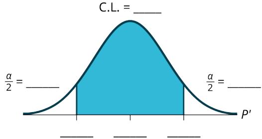
Figure B.5.1 — The picture behind every confidence interval for a proportion. The shaded middle is the confidence level, the two unshaded tails each hold \(\frac{\alpha}{2}\), and the three blanks on the horizontal axis take the lower limit, the sample proportion \(p'\), and the upper limit, left to right.
The confidence level and \(\alpha\) are two ways of saying the same thing, and the graph makes the relationship visible. The shaded region is the confidence level, so a 90% interval shades 0.90 and leaves \(\alpha = 1 - 0.90 = 0.10\) unshaded. That leftover area is split evenly between the two tails because the interval reaches the same distance in both directions, which puts \(\frac{\alpha}{2} = 0.05\) in each one. When you go looking up a \(z\)-value in a table or a calculator, the number you need is keyed to that tail area, not to the confidence level itself, and mixing the two up is the single most common way this calculation goes wrong. Write \(\alpha\) and \(\frac{\alpha}{2}\) down before you look anything up.
Try it in rāSHio
Once your class has its two counts, the whole interval is one tool call. In rāSHio, choose Stats → Prop Stats, untick Hypothesis Test and tick Confidence Interval, then enter your successes, your sample size, and whichever confidence level you want; it reports \(p'\), the error bound, and both endpoints together. Run it at 0.90 for the items above, then run it again at each level in Table B.5.1 — changing that one field is the whole of question 3, and watching the endpoints move while the centre holds still is the answer to question 4.
Figure B.5.2 — Prop Stats in Confidence Interval mode: successes, sample size, confidence level in, interval out. Watch step 3, where Hypothesis Test is unticked — that checkbox is what decides which of the two procedures the dialog runs. The walkthrough uses its own demonstration counts at the 0.95 level, which is one of the rows Table B.5.1 asks you for, not your class’s counts at 0.90.
Using Diego's class of 40 with 26 students born in this state, calculate the error bound and the 90% confidence interval.
Solution — the ninety percent interval
Step 1 — find the standard error.
$$ \sqrt{\frac{p'q'}{n}} = \sqrt{\frac{(0.65)(0.35)}{40}} = \sqrt{0.0056875} \approx 0.0754 $$Step 2 — find the critical value. For 90% confidence, \(\alpha = 0.10\) and \(\frac{\alpha}{2} = 0.05\), so
$$ z_{\frac{\alpha}{2}} = z_{0.05} = 1.645 $$Step 3 — compute the error bound.
$$ EBP = (1.645)(0.0754) \approx 0.1241 $$Step 4 — build the interval.
$$ \left(0.6500 - 0.1241,\ 0.6500 + 0.1241\right) = (0.5259,\ 0.7741) $$Answer: \(EBP \approx 0.1241\) and the 90% confidence interval is \((0.5259,\ 0.7741)\). That interval is about a quarter of the whole scale wide, which is what forty students buys you. It is a real answer, and it is also a reminder that a small sample cannot pin a proportion down tightly no matter how carefully you do the arithmetic.
Hannah Whitfield is labelling Figure B.5.1 for the same 90% interval Diego built. State the \(\alpha\) and \(\frac{\alpha}{2}\) she needs, then say exactly what goes in each of the five blanks on her graph.
Solution — labelling the tail areas and the axis
Step 1 — find the total tail area. The confidence level is 0.90, so
$$ \alpha = 1 - 0.90 = 0.10 $$Step 2 — split it between the two tails.
$$ \frac{\alpha}{2} = \frac{0.10}{2} = 0.05 $$Step 3 — fill in the graph. The label at the top of the curve is the confidence level, so C.L. = 0.90. The two \(\frac{\alpha}{2}\) blanks, one on each side, both take 0.05. The three blanks under the horizontal axis take the interval's lower limit, the sample proportion, and the upper limit, left to right: 0.5259, 0.6500, 0.7741.
Answer: \(\alpha = 0.10\), \(\frac{\alpha}{2} = 0.05\), the shaded centre is labelled 0.90, and the number line reads 0.5259, 0.6500, 0.7741. Check the three axis values before you move on: the middle one must be exactly halfway between the outer two, because the interval was built by stepping the same distance out in both directions. If it is not, one of the two endpoints has an arithmetic error in it.
B.5.4 Describe the Confidence Interval
The confidence level of an interval is the proportion of intervals, built this same way from repeated samples of the same size, that would contain the true population proportion \(p\).
Widening an interval until you are 99% sure is easy — say the proportion is somewhere between 0 and 1 and you are 100% sure. The useful interval is the narrow one you can still defend, which is why nobody reports a 99.99% interval.
Read that carefully, because it is a statement about the method rather than about your one interval. Your interval either contains \(p\) or it does not; there is nothing random left in it once the data are collected. What is 90% is the long-run success rate of the procedure that produced it.
Now put the interval into words, and then find out what changing the confidence level does to it.
- In two to three complete sentences, explain what a confidence interval means (in general), as though you were talking to someone who has not taken statistics.
- In one to two complete sentences, explain what this confidence interval means for this particular study.
- Construct a confidence interval for each confidence level given.
| Confidence level | EBP / Error Bound | Confidence Interval |
|---|---|---|
| 50% | ||
| 80% | ||
| 95% | ||
| 99% |
- What happens to the \(EBP\) as the confidence level increases? Does the width of the confidence interval increase or decrease? Explain why this happens.
Only one quantity in the error bound formula changes as you move down Table B.5.1. Your class collected one set of data, so \(p'\), \(q'\), and \(n\) are fixed, which means the standard error \(\sqrt{\frac{p'q'}{n}}\) is the same 0.0754 in every row. The whole table is that one number multiplied by five different critical values. Once you see it that way, question 4 stops being a question about statistics and becomes a question about the \(z\)-values: they get larger as you ask for more confidence, and everything else follows.
Try it in rāSHio
The five critical values are the only thing Table B.5.1 needs that your data cannot supply, and Distributions → Normal in rāSHio will give you each one. Set the mean to 0 and the standard deviation to 1, then use the inverse lookup: ask for the value with \(1 - \frac{\alpha}{2}\) of the area to its left, so a 95% interval asks for 0.975 and returns 1.96. Do that once per row and the rest of the table is a single multiplication.
Answer questions 1 and 2 for Diego's class of 40 with a 90% interval of \((0.5259,\ 0.7741)\).
Solution — explaining an interval in plain words
Step 1 — the general explanation. A confidence interval is a range of plausible values for something you cannot measure directly, built from a sample you can measure. The confidence level tells you how often this way of building ranges gets it right: if you took many different samples the same size and built a range from each one, about 90% of those ranges would contain the true value. It does not tell you the chance that this one particular range is correct, because that range is already fixed once the data are in.
Step 2 — the explanation for this study. We are 90% confident that between 52.59% and 77.41% of all students at this school were born in this state.
Answer: the general version describes the reliability of the procedure across many samples; the study-specific version names the population, the quantity, and the two endpoints in one sentence. Watch the wording in step 2: the claim is about all students at this school, not about the 40 who were surveyed. The proportion for those 40 is not estimated and not uncertain — it is 0.65, and we counted it.
Complete Table B.5.1 for Diego's class of 40, then answer question 4.
Solution — four confidence levels compared
Step 1 — hold the standard error fixed. The data do not change, so every row uses \(\sqrt{\frac{p'q'}{n}} \approx 0.0754\) and every interval is centred at \(p' = 0.6500\).
Step 2 — look up the critical value for each level and multiply.
$$ EBP_{50\%} = (0.6745)(0.0754) \approx 0.0509 \qquad EBP_{80\%} = (1.282)(0.0754) \approx 0.0967 $$ $$ EBP_{95\%} = (1.960)(0.0754) \approx 0.1478 \qquad EBP_{99\%} = (2.576)(0.0754) \approx 0.1943 $$Step 3 — step out from 0.6500 in both directions.
| Confidence level | \(z_{\frac{\alpha}{2}}\) | EBP | Confidence interval | Width |
|---|---|---|---|---|
| 50% | 0.6745 | 0.0509 | (0.5991, 0.7009) | 0.1017 |
| 80% | 1.282 | 0.0967 | (0.5533, 0.7467) | 0.1933 |
| 90% | 1.645 | 0.1241 | (0.5259, 0.7741) | 0.2481 |
| 95% | 1.960 | 0.1478 | (0.5022, 0.7978) | 0.2956 |
| 99% | 2.576 | 0.1943 | (0.4557, 0.8443) | 0.3885 |
Step 4 — answer question 4. As the confidence level increases, the \(EBP\) increases and the interval gets wider. The reason is that \(p'\), \(q'\), and \(n\) never move, so the standard error is the same in every row; the only thing that changes is \(z_{\frac{\alpha}{2}}\), which grows as you ask for more confidence. Asking for more confidence means demanding that more of the area under the curve fall inside your interval, and the only way to capture more area is to reach further out from the centre in both directions.
Answer: the error bound rises from 0.0509 to 0.1943 and the width rises from 0.1017 to 0.3885 as the confidence level goes from 50% to 99%. The 50% interval is the one worth staring at. It is narrow and precise, and it is wrong half the time. Precision that you cannot trust is not an improvement, which is why nobody reports a 50% interval even though it looks like the best answer in the table.
Key Terms
confidence interval — a range of values, computed from a sample, that is used to estimate an unknown population parameter.
confidence level — the proportion of intervals built this way from repeated samples that would contain the true parameter; equal to \(1 - \alpha\).
error bound for a proportion (EBP) — the distance from the sample proportion to either endpoint of the interval, \(EBP = z_{\frac{\alpha}{2}}\sqrt{\frac{p'q'}{n}}\).
sample proportion — the number of successes divided by the sample size, \(p' = \frac{x}{n}\); its complement is \(q' = 1 - p'\).
standard error of a proportion — \(\sqrt{\frac{p'q'}{n}}\), the typical distance between a sample proportion and the population proportion.