12.1 One-Way ANOVA
SLO 4
Demonstrate an understanding of, and ability to use, basic ideas of statistical processes, including hypothesis tests and confidence interval estimation.
SLO 5
Identify appropriate statistical techniques and use technology-based statistical analysis to describe, interpret, and communicate results.
Learning Objectives
By the end of this section, you will be able to:
- explain what question a one-way ANOVA test answers and why it uses variances to compare means;
- list and check the five assumptions a data set must satisfy before a one-way ANOVA can be performed;
- write the null and alternative hypotheses for a one-way ANOVA test with any number of groups;
- interpret side-by-side box plots to judge whether group mean differences look like random variation or something real.
12.1.1 What a One-Way ANOVA Does
Suppose you want to know whether three different study methods lead to different average exam scores. You could run a two-sample test comparing method A against method B, then another comparing A against C, then another comparing B against C. But every test you run adds another chance of a false alarm, and by the time you have compared all the pairs, your overall error rate has quietly ballooned. The one-way ANOVA solves this by answering all of those questions at once with a single test.
Each pairwise test carries roughly a 5% chance of a false positive. With four groups there are six pairs, so the chance that at least one comparison "finds" a difference that isn't really there climbs past 25%. ANOVA keeps the error rate under control by testing everything in one shot.
The purpose of a one-way ANOVA test is to determine the existence of a statistically significant difference among several group means. Here is the surprising part: even though we care about means, the test actually uses variances to help decide if the means are equal or not. It compares two kinds of variation — how much the group averages differ from each other, versus how much individual values bounce around within each group. If the variation between groups is large compared to the variation within groups, the means probably are not all equal.
The name tells you the structure. "One-way" means there is exactly one factor — one characteristic that splits the data into groups. Study method is a factor with three groups (A, B, C). If you also split students by, say, class year, you would need a two-way ANOVA, which is beyond this section.
A one-way ANOVA (analysis of variance) is a hypothesis test used to determine whether a statistically significant difference exists among the means of several groups, where the groups are defined by a single categorical factor.
In plain terms: one-way ANOVA asks, "Do these several groups all come from populations with the same average, or is at least one average different?" — and it answers using variances rather than direct mean-to-mean comparisons.
Two vocabulary words will keep coming up, so let's pin them down now.
Definition 12.1.1 — One-Way ANOVA: One-way ANOVA answers by comparing variances, not mean-to-mean pairs.
The factor is the categorical variable that separates the data into the groups being compared. In the study-method example, the factor is "study method," and its values (method A, method B, method C) are the groups.
Definition 12.1.2 — Factor: The factor's values are the groups being compared.
The response variable is the numerical quantity we measure on each subject — the thing whose means we are comparing. In the study-method example, the response variable is the exam score.
Think of the factor as the label on each mailbox and the response as the mail inside. ANOVA asks whether the average amount of mail differs from box to box by more than day-to-day jitter within a single box would explain.
You will meet this test again throughout the chapter, so it helps to keep the big picture in view from the start. Every one-way ANOVA has the same skeleton: one categorical factor that sorts subjects into \(k\) groups, one numerical response measured on every subject, and one question — are all \(k\) population means equal? Everything else in this section (the assumptions, the hypotheses, the box plots) exists to set up that single question carefully before any arithmetic happens.
Definition 12.1.3 — Response Variable: One factor sorts subjects into groups; the response is what we measure on every subject in every group.
12.1.2 The Five Assumptions
Before you can trust a one-way ANOVA result, five conditions must hold. Check them before running the test — an ANOVA run on data that violates its assumptions can hand you a confident answer to a question the test cannot actually address.
- Normality. Each population from which a sample is taken is assumed to be normal.
- Random, independent samples. All samples are randomly selected and independent of one another.
- Equal standard deviations. The populations are assumed to have equal standard deviations (or equivalently, equal variances).
- Categorical factor. The factor is a categorical variable.
- Numerical response. The response is a numerical variable.
Let's unpack what each one means in practice:
- Assumption 1 (normality): whatever population each sample comes from should follow a bell-shaped distribution. With moderate sample sizes, ANOVA tolerates modest departures, but badly skewed populations undermine the test.
- Assumption 2 (random and independent): randomness protects against bias in who or what ends up in each group, and independence means one observation tells you nothing about another — no repeated measures on the same subjects, no clusters.
- Assumption 3 (equal spread): each population should have roughly the same standard deviation. This matters because the whole machinery of ANOVA pools the within-group variation; if one group's spread dwarfs the others, that pooling misleads.
- Assumptions 4 and 5 (variable types): the grouping variable must be categories (like brand, treatment, or location), and the measured variable must be numbers (like weight, time, or score). That combination — categories defining groups, numbers measuring outcomes — is exactly the shape of data one-way ANOVA is built for.
Notice how assumptions 4 and 5 work together. They describe the form of your data table: one column of group labels drawn from a short list of categories, and one column of numbers. If either column has the wrong type — group labels that are really measurements, or responses that are really rankings rather than quantities — the test does not fit the question.
Running ANOVA on data with wildly unequal spreads is like averaging gas prices across towns where some prices are quoted per gallon and others per liter — the arithmetic runs fine, but the result answers a question nobody asked.
A quick habit worth building: when you meet a new data set, run through the five assumptions as a checklist before anything else. Two of them (4 and 5) you can verify instantly by looking at the variables. The other three require judgment about how the data were collected and what the populations look like — and that judgment gets easier with practice, like the exercise below.
For each scenario, decide whether one-way ANOVA is appropriate, and if not, say which assumption fails.
a) A researcher measures the cholesterol levels (mg/dL) of randomly selected patients at four independent clinics and wants to know whether the clinics' average cholesterol levels differ.
b) A teacher sorts students into three groups by favorite pizza topping and compares their heights.
c) A company surveys customers once per year for five years and wants to compare average satisfaction scores, treating each customer's yearly scores as separate observations.
Solution
a) Yes. The factor (clinic) is categorical, the response (cholesterol level) is numerical, samples are random and independent, and the standard assumptions of normality and equal standard deviations are the ones we would check in the data. All five assumptions are plausibly met.
b) No — this fails the spirit of the design. Pizza topping preference is indeed categorical and height is numerical, but there is no reason to expect the populations to be normal with equal standard deviations, and more importantly the grouping has no meaningful experimental basis. Technically the variable-type assumptions (4 and 5) hold, but assumptions 1–3 about the populations cannot be reasonably claimed. ANOVA is not the right tool here.
c) No — assumption 2 fails. The same customer's scores across years are not independent observations; they are repeated measures on the same people. Treating them as independent inflates the effective sample size and invalidates the test.
12.1.3 The Null and Alternative Hypotheses
Every hypothesis test starts with two competing claims, and ANOVA's pair is refreshingly simple.
The null hypothesis says all the group population means are the same — every group is really drawing from a population with the same average, and any differences we see in the samples are just random noise. The alternative hypothesis says at least one pair of means is different.
If there are \(k\) groups, we write the null hypothesis as:
$$H_0: \mu_1 = \mu_2 = \mu_3 = \dots = \mu_k$$and the alternative as:
$$H_a: \text{At least two of the group means } \mu_1, \mu_2, \mu_3, \ldots, \mu_k \text{ are not equal.}$$That is, \(\mu_i \neq \mu_j\) for some \(i \neq j\).
Notice what the alternative does not say. It does not claim that all the means differ from one another, and it does not tell you which ones differ. It only asserts that the "all equal" story is broken somewhere. If we reject \(H_0\), further analysis is needed to find which pair or pairs disagree — that follow-up work comes later in the chapter.
For a one-way ANOVA with \(k\) groups, the null hypothesis is \(H_0: \mu_1 = \mu_2 = \mu_3 = \dots = \mu_k\) — all \(k\) population means are equal.
Definition 12.1.4 — Null Hypothesis for One-Way ANOVA: All k population means are equal.
The alternative hypothesis is \(H_a:\) at least two of the group means \(\mu_1, \mu_2, \mu_3, \ldots, \mu_k\) are not equal; that is, \(\mu_i \neq \mu_j\) for some \(i \neq j\).
Writing these hypotheses correctly is mostly bookkeeping, but small slips change the meaning of the whole test. Three habits keep you safe: label the means with subscripts matching your groups (\(\mu_1\) for group 1, and so on), always chain the null with equal signs across all \(k\) groups, and never turn the alternative into "all means differ." The next example walks through the full process.
Definition 12.1.5 — Alternative Hypothesis for One-Way ANOVA: Rejecting H₀ breaks the "all equal" story somewhere — it does not say which pair, and it never claims that all k means differ from one another.
A gardener tests four fertilizer brands (W, X, Y, Z) and records tomato yield in pounds per plant. Write the null and alternative hypotheses for a one-way ANOVA.
Solution
Here \(k = 4\), so we label the four population mean yields \(\mu_W, \mu_X, \mu_Y, \mu_Z\).
Step 1 — Identify the groups and their means: the factor is fertilizer brand, with four categories, so there are four population mean yields to compare.
Null hypothesis: all four brands produce the same average yield.
$$H_0: \mu_W = \mu_X = \mu_Y = \mu_Z$$Alternative hypothesis: at least one pair of brands differs in average yield.
$$H_a: \text{At least two of } \mu_W, \mu_X, \mu_Y, \mu_Z \text{ are not equal.}$$Note that \(H_a\) does not say all four differ — maybe only brand Y stands apart. The alternative just denies complete equality.
A hospital network wants to know whether average patient wait times differ among its five emergency rooms. Let \(\mu_1, \mu_2, \mu_3, \mu_4, \mu_5\) be the five population mean wait times.
a) State \(H_0\) and \(H_a\) for this test.
b) Suppose the test rejects \(H_0\). Does that prove all five wait-time means are different from each other? Explain.
Solution
a) With \(k = 5\):
$$H_0: \mu_1 = \mu_2 = \mu_3 = \mu_4 = \mu_5$$\(H_a:\) At least two of \(\mu_1, \mu_2, \mu_3, \mu_4, \mu_5\) are not equal; that is, \(\mu_i \neq \mu_j\) for some \(i \neq j\).
b) No. Rejecting \(H_0\) supports only the alternative claim — that at least one pair of means differs. It might be that four ERs share the same average while one lags behind. Identifying which means differ requires additional analysis after the ANOVA.
12.1.4 Reading the Box Plots
Box plots give you a visual preview of what the ANOVA is deciding. Draw one box plot per group, side by side on the same scale, with each group's mean marked by a horizontal line through the box. Then ask one question: do the mean lines sit close together, relative to how much the data spread within each box?
If the null hypothesis is true — say \(H_0: \mu_1 = \mu_2 = \mu_3\) for three groups — then all three populations have the same distribution, and the three mean lines should sit at roughly the same height. In that case, the variance of the combined data (all groups lumped together) is approximately the same as the variance of each individual population. Lumping changes nothing because the groups are interchangeable.
If the null hypothesis is false, the picture changes. The group means sit at noticeably different heights, and when you pool the data, the combined variance becomes larger than any single population's variance. Why? Because the pooled cloud now stretches across groups centered at different places — the separation between the means itself adds spread. That extra between-group spread is exactly the signal ANOVA detects.
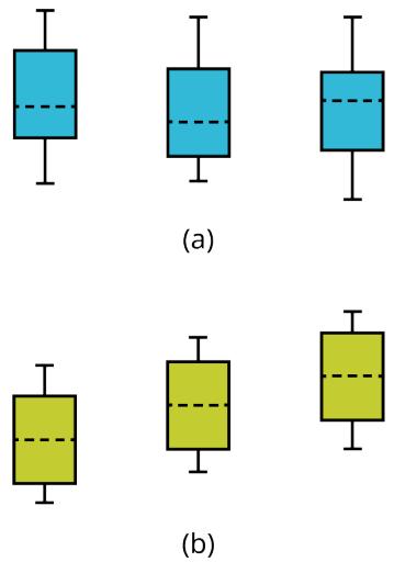
Figure 12.1.1 — (a) \(H_0\) is true. All means are the same; the differences are due to random variation. (b) \(H_0\) is not true. The means are not all the same; the differences are too large to be due to random variation.
Look at panel (a): the three blue box plots have mean lines at essentially the same level, and the boxes overlap heavily. Any wobble among the sample means is small enough to attribute to chance. Panel (b) shows green box plots whose mean lines are clearly separated — the gaps between them are too large to blame on random variation alone, which is why the combined-data variance swells.
Total scatter in the pooled data = scatter within each group + scatter caused by the group means sitting at different heights. When the second piece grows big enough next to the first, ANOVA flags it.
This visual intuition is exactly what the formal test quantifies: it computes how much of the total variation comes from differences between group means and compares that to the variation left over within groups. The next sections carry out that computation.
Before moving on, practice reading the picture the way the test will read it. The key comparison is always the same: the gaps between mean lines versus the width of the boxes themselves. Wide boxes with close mean lines suggest chance; narrow boxes with far-apart mean lines suggest real differences.
Three call centers record their daily handling times. In scenario A, side-by-side box plots show mean lines at 6.1, 6.3, and 6.2 minutes, with boxes spanning roughly 4 to 9 minutes and heavy overlap. In scenario B, the same three centers show mean lines at 4.5, 6.2, and 8.0 minutes, with boxes of similar width to scenario A.
a) Which scenario looks consistent with \(H_0\)?
b) In which scenario would you expect the variance of the combined data to be noticeably larger than the variance within each group?
Solution
a) Scenario A. The mean lines (6.1, 6.3, 6.2) sit nearly at the same height and the boxes overlap heavily, so the observed differences among sample means are small enough to be explained by random variation — the picture matches \(H_0: \mu_1 = \mu_2 = \mu_3\).
b) Scenario B. With means at 4.5, 6.2, and 8.0 minutes, pooling the three groups produces a data cloud stretched far wider than any single group's own spread. The between-mean separation inflates the combined variance well above each population's variance — the signature of a false \(H_0\).
Problem Set 12.1
Problem 1. State in one sentence what question a one-way ANOVA answers.
Solution
Step 1 — Identify the core question: A one-way ANOVA asks whether a statistically significant difference exists among the means of several groups defined by a single categorical factor.
Answer: One-way ANOVA answers the question: "Do all of these groups come from populations with the same mean, or is at least one group's mean different?"
Problem 2. Explain why running every pairwise two-sample test instead of one ANOVA is a problem. Use the phrase "error rate" in your answer.
Solution
Step 1 — Count the tests: With several groups there are many pairs to compare (e.g., four groups give six pairwise comparisons), so running a two-sample test for every pair means many separate hypothesis tests.
Step 2 — Explain the error-rate problem: Each individual test carries roughly a 5% chance of a false positive, and these chances accumulate: across many tests, the overall error rate — the probability that at least one comparison falsely "finds" a difference — balloons well past 5% (past 25% with four groups).
Step 3 — State ANOVA's advantage: One-way ANOVA answers all the group-mean questions in a single test, keeping the overall error rate under control.
Answer: Running every pairwise test multiplies the chances of a false alarm, so the overall error rate climbs far above the intended level; a single ANOVA avoids this by testing all the means at once.
Problem 3. A one-way ANOVA compares means. Explain why it does so by looking at variances.
Solution
Step 1 — Identify the two kinds of variation: The test compares how much the group averages differ from each other (variation between groups) against how much individual values bounce around within each group (variation within groups).
Step 2 — Explain the logic: If \(H_0\) is true and all population means are equal, the between-group differences are no larger than ordinary within-group random variation would produce. If the between-group variation is large relative to the within-group variation, the means probably are not all equal.
Step 3 — Connect to combined variance: When the means are equal, pooling the data leaves the variance unchanged; when the means are spread apart, the pooled (combined) variance grows because the separation between group centers adds extra spread.
Answer: ANOVA uses variances because the ratio of between-group to within-group variation reveals whether observed mean differences exceed what random variation alone would explain.
Problem 4. List the five assumptions required for a one-way ANOVA.
Solution
Step 1 — List assumptions 1–3 about the populations and samples: (1) Each population from which a sample is taken is normal; (2) all samples are randomly selected and independent of one another; (3) the populations have equal standard deviations (equal variances).
Step 2 — List assumptions 4–5 about variable types: (4) The factor is a categorical variable; (5) the response is a numerical variable.
Answer: The five assumptions are: (1) normality of each population, (2) random and independent samples, (3) equal standard deviations across populations, (4) a categorical factor, and (5) a numerical response.
Problem 5. For each situation, name the factor and the response variable. a) Comparing average battery life across four phone brands. b) Comparing average germination time for seeds kept at three temperatures.
Solution
a)
Step 1 — Identify the grouping variable: Phone brand is a categorical variable with four categories, so it is the factor.
Step 2 — Identify the measured quantity: Battery life is a numerical measurement taken on each phone, so it is the response variable.
b)
Step 1 — Identify the grouping variable: Temperature setting is categorical with three levels, so it is the factor.
Step 2 — Identify the measured quantity: Germination time is a numerical measurement on each seed, so it is the response variable.
Answer: a) Factor = phone brand; response = battery life. b) Factor = temperature; response = germination time.
Problem 6. Explain what the word "one-way" refers to in "one-way ANOVA."
Solution
Step 1 — Recall what splits the data into groups: The factor is the single categorical variable that defines the groups being compared.
Step 2 — Apply it to the name: "One-way" means there is exactly one factor — one characteristic sorting subjects into groups. (If two characteristics each split the data, you would need a two-way ANOVA.)
Answer: "One-way" refers to the presence of exactly one categorical factor defining the groups.
Problem 7. A study measures reaction times of the same twelve people under three lighting conditions. Which assumption does this design violate, and why?
Solution
Step 1 — Examine the design: The same twelve people are measured under all three lighting conditions, so each person contributes three related observations.
Step 2 — Match to the assumptions: Assumption 2 requires all samples to be randomly selected and independent of one another. Repeated measures on the same subjects are not independent — one person's reaction time under one condition tells you something about their time under another condition.
Answer: This design violates assumption 2 (random, independent samples), because measuring the same twelve people under all three conditions produces repeated measures rather than independent observations.
Problem 8. Write \(H_0\) and \(H_a\) for a one-way ANOVA comparing the mean weekly hours studied by students in six different majors.
Solution
Step 1 — Count the groups: There are six majors, so \(k = 6\), and we label the population mean weekly study hours \(\mu_1\) through \(\mu_6\).
Step 2 — Write the null hypothesis: All six population means are equal:
$$H_0: \mu_1 = \mu_2 = \mu_3 = \mu_4 = \mu_5 = \mu_6$$Step 3 — Write the alternative hypothesis: At least one pair of means differs:
$$H_a: \text{At least two of } \mu_1, \mu_2, \mu_3, \mu_4, \mu_5, \mu_6 \text{ are not equal.}$$Answer: \(H_0: \mu_1 = \mu_2 = \mu_3 = \mu_4 = \mu_5 = \mu_6\); \(H_a:\) at least two of the six means are not equal (\(\mu_i eq \mu_j\) for some \(i eq j\)).
Problem 9. A classmate writes the alternative hypothesis as \(H_a: \mu_1 \neq \mu_2 \neq \mu_3\). Explain what is wrong with this and write it correctly.
Solution
Step 1 — Diagnose the classmate's version: Writing \(H_a: \mu_1 eq \mu_2 eq \mu_3\) reads like a chain claiming all the means differ from one another. That overstates the alternative: rejecting \(H_0\) only means at least one pair differs — perhaps just one group stands apart while the other two agree.
Step 2 — Write it correctly: State the alternative as a denial of complete equality, not as universal inequality:
$$H_a: \text{At least two of } \mu_1, \mu_2, \mu_3 \text{ are not equal.}$$That is, \(\mu_i eq \mu_j\) for at least one pair \(i eq j\).
Answer: The chained form wrongly claims all three means differ from each other; correctly, \(H_a\) states only that at least two of \(\mu_1, \mu_2, \mu_3\) are not equal.
Problem 10. An ANOVA rejects \(H_0\) for four groups. State precisely what has and has not been established.
Solution
Step 1 — State what has been established: Rejecting \(H_0\) establishes that the null claim of complete equality is unsupported — that is, at least one pair of the four group means differs significantly.
Step 2 — State what has NOT been established: We have not established that all the means differ from one another, nor have we identified which pair or pairs differ. Some of the four means may still be equal.
Answer: Rejection establishes only that at least two of the four group means are not equal; it does not show which ones differ or that all four differ — follow-up analysis is needed for that.
Problem 11. Side-by-side box plots for three groups show mean lines at nearly the same height but very narrow boxes. Explain what this picture suggests and why the width of the boxes matters to the comparison.
Solution
Step 1 — Read the mean lines: Mean lines at nearly the same height suggest the sample means are close together, which is consistent with \(H_0: \mu_1 = \mu_2 = \mu_3\) being true.
Step 2 — Explain why box width matters: Very narrow boxes mean little within-group variation, so even small gaps between means would be hard to attribute to chance. Here the gaps are tiny relative to nothing much — but the key comparison is always gap size versus box width. Narrow boxes make the test sensitive: if the mean lines were separated even modestly, that separation would be strong evidence of real differences, because narrow boxes indicate small random variation to blame it on.
Answer: The picture suggests the group means are essentially equal (consistent with \(H_0\)); the narrow boxes matter because they show within-group variation is small, so any visible separation of mean lines would be meaningful evidence against \(H_0\).
Problem 12. Explain in one or two sentences why the variance of the combined data grows when the group means are far apart.
Solution
Step 1 — Recall what pooling does: The combined-data variance measures spread around the overall average of all groups lumped together.
Step 2 — Explain the effect of separated means: When group means sit far apart, each group clusters around its own center, and those centers are scattered widely. The pooled cloud therefore stretches across all the different group locations, so the total spread includes both the within-group scatter and the spread caused by the differing means.
Answer: Far-apart group means add between-group spread on top of within-group scatter when the data are pooled, so the combined variance becomes noticeably larger than any single population's variance.
Key Terms
one-way ANOVA — a hypothesis test that determines whether a statistically significant difference exists among the means of several groups defined by a single categorical factor, using variances to make the decision.
factor — the categorical variable that separates the data into the groups being compared.
response variable — the numerical quantity measured on each subject, whose group means the test compares.
null hypothesis (\(H_0\)) — the claim that all \(k\) group population means are equal: \(\mu_1 = \mu_2 = \dots = \mu_k\).
alternative hypothesis (\(H_a\)) — the claim that at least two of the group means are not equal; \(\mu_i \neq \mu_j\) for some \(i \neq j\).
combined variance — the variance computed from all groups pooled together; approximately equal to each population's variance when \(H_0\) is true, and larger when the group means truly differ.