12.3 Facts About the F Distribution
SLO 4
Demonstrate an understanding of, and ability to use, basic ideas of statistical processes, including hypothesis tests and confidence interval estimation.
SLO 5
Identify appropriate statistical techniques and use technology-based statistical analysis to describe, interpret, and communicate results.
Learning Objectives
By the end of this section, you will be able to:
- describe the key properties of the F distribution, including its shape and how it changes with the degrees of freedom;
- carry out a complete one-way ANOVA hypothesis test, from stating hypotheses to writing a conclusion;
- build an ANOVA table by computing sums of squares, mean squares, and the F statistic;
- use a TI-83/84 calculator to run ANOVA and to find p-values with the Fcdf command.
12.3.1 Here Are Some Facts About the F Distribution
Before we run any tests with it, let's get comfortable with what the F distribution actually looks like. Here are the facts you need:
- The curve is not symmetrical but skewed to the right.
- There is a different curve for each set of dfs.
- The F statistic is greater than or equal to zero.
- As the degrees of freedom for the numerator and for the denominator get larger, the curve approximates the normal.
- Other uses for the F distribution include comparing two variances and two-way Analysis of Variance. Two-Way Analysis is beyond the scope of this chapter.
Think of the F distribution like a right-skewed income curve: most values pile up near zero on the left, with a long tail stretching right. That tail is exactly where large F statistics land when group means really do differ — so a big F means a small p-value.
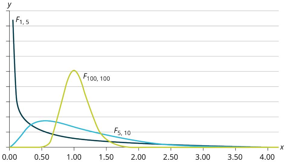
Figure 12.3.1 — Three F curves showing how shape depends on degrees of freedom.
Notice in Figure 12.3.1 how different the three curves are. With \(F_{100,100}\) — both degrees of freedom large — the curve is tall and humped like a normal curve, centered near 1. With \(F_{1,5}\), almost all the area sits near zero. Each pair of dfs gives its own curve, which is why we always report \(F\) with two subscripts.
Decide whether each statement about the F distribution is true or false, and say which of the five facts settles it.
a) An F statistic of \(-0.4\) means the within-group variation was larger than the between-group variation.
b) \(F_{3,20}\) and \(F_{20,3}\) describe the same curve.
c) As both degrees of freedom grow, the F curve looks more and more like a normal curve.
Solution — reading the properties, not the picture
a) False. Fact 3 says the F statistic is greater than or equal to zero. It is a ratio of two mean squares, and a mean square is built from squared deviations, so neither part can be negative. A negative F means an arithmetic error, not a small between-group variation. (When the within-group variation is larger, F comes out between 0 and 1 — still positive.)
b) False. Fact 2 says there is a different curve for each set of degrees of freedom, and the two dfs are not interchangeable: the first counts groups minus one, the second counts observations minus groups. \(F_{3,20}\) and \(F_{20,3}\) are different curves.
c) True. That is fact 4 exactly. With both dfs large, the sharp right skew flattens out and the curve approaches a normal shape centred near 1.
Answer: a) False, b) False, c) True.
12.3.2 Running a Complete ANOVA Test
The facts above describe the distribution. Now we use it. The next three sections each work a full test start to finish — state the hypotheses, build the ANOVA table, find the p-value, and write the conclusion — on a different kind of data set.
There are multiple variants of the virus that causes COVID-19. The length of hospital stays for patients afflicted with various strains of COVID-19 is shown in Table 12.3.1.
| Delta Strain | Omicron Strain | Alpha Strain | Gamma Strain | Beta Strain |
|---|---|---|---|---|
| 13.9 | 11.7 | 18.2 | 16.9 | 9.3 |
| 14.9 | 15.1 | 14.6 | 12.8 | 15.8 |
| 16.8 | 9.9 | 10.1 | 11.2 | 16.4 |
Test whether the mean length of hospital stay is the same or different for the various strains of COVID-19. Construct the ANOVA table, find the p-value, and state your conclusion. Use a 5% significance level.
Solution
Hypotheses: \(H_0: \mu_1 = \mu_2 = \mu_3 = \mu_4 = \mu_5\) versus \(H_a:\) at least two of the strain means differ.
Group means: Delta = 15.2, Omicron = 12.2333, Alpha = 14.3, Gamma = 13.6333, Beta = 13.8333.
Grand mean: \(\bar{x} = 13.84\). Total sample size \(n = 15\), number of groups \(k = 5\).
SS(Between) \(= 3[(15.2 - 13.84)^2 + (12.2333 - 13.84)^2 + (14.3 - 13.84)^2 + (13.6333 - 13.84)^2 + (13.8333 - 13.84)^2] \approx 3[1.8496 + 2.5814 + 0.2116 + 0.0427 + 0.00005] \approx 14.06\)
SS(Within): group variances are Delta ≈ 2.17, Omicron ≈ 6.97, Alpha ≈ 16.47, Gamma ≈ 8.64, Beta ≈ 15.50. Sum × 2 df each: \(2(2.17 + 6.97 + 16.47 + 8.64 + 15.50) \approx 99.52\)
SS(Total) ≈ 113.58 (check: 14.06 + 99.52 = 113.58 ✓)
| Source | SS | df | MS | F |
|---|---|---|---|---|
| Factor (Between) | ≈ 14.06 | 5 − 1 = 4 | ≈ 3.51 | \(\frac{3.51}{9.95} \approx 0.353\) |
| Error (Within) | ≈ 99.52 | 15 − 5 = 10 | ≈ 9.95 | |
| Total | ≈ 113.58 | 14 |
Distribution: \(F_{4,10}\); test statistic \(F \approx 0.353\).
p-value: \(P(F > 0.353) \approx 0.84\).
Decision: Since p-value = 0.84 > \(\alpha = 0.05\), do not reject \(H_0\).
Conclusion: At the 5% significance level, there is not sufficient evidence to conclude that the mean length of hospital stay differs among the strains of COVID-19.
Let's return to the slicing tomato exercise from Try It Now 12.8 in the previous section. The means of the tomato yields under the five mulching conditions are represented by \(\mu_1, \mu_2, \mu_3, \mu_4, \mu_5\). We will conduct a hypothesis test to determine if all means are the same or at least one is different. Using a significance level of 5%, test the null hypothesis that there is no difference in mean yields among the five groups against the alternative hypothesis that at least one mean is different from the rest.
Solution
Step 1 — State the hypotheses.
$$H_0: \mu_1 = \mu_2 = \mu_3 = \mu_4 = \mu_5$$ $$H_a: \mu_i \neq \mu_j \text{ some } i \neq j$$The null says every mulch produces the same average yield. The alternative says at least one mulch differs from the others — not that all differ.
Step 2 — Build the ANOVA table.
| Source of Variation | Sum of Squares (SS) | Degrees of Freedom (df) | Mean Square (MS) | F |
|---|---|---|---|---|
| Factor (Between) | 36,648,561 | 5 − 1 = 4 | \(\frac{36,648,561}{4} = 9,162,140\) | \(\frac{9,162,140}{2,044,672.6} = 4.4810\) |
| Error (Within) | 20,446,726 | 15 − 5 = 10 | \(\frac{20,446,726}{10} = 2,044,672.6\) | |
| Total | 57,095,287 | 15 − 1 = 14 |
Step 3 — Identify the distribution. Distribution for the test: \(F_{4,10}\)
$$df(num) = 5 - 1 = 4$$ $$df(denom) = 15 - 5 = 10$$Test statistic: \(F = 4.4810\)
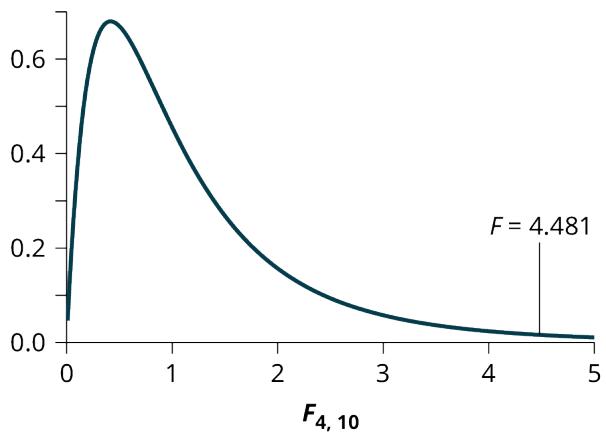
Figure 12.3.2 — The \(F_{4,10}\) curve with the test statistic marked.
Step 4 — Find the p-value. Probability Statement: p-value = \(P(F > 4.481) = 0.0248\).
Step 5 — Compare α and the p-value: \(\alpha = 0.05\), p-value = 0.0248.
Step 6 — Make a decision: Since \(\alpha >\) p-value, we reject \(H_0\).
Answer: At the 5% significance level, we have reasonably strong evidence that differences in mean yields for slicing tomato plants grown under different mulching conditions are unlikely to be due to chance alone. We may conclude that at least some of the mulches led to different mean yields.

Figure 12.3.3 — TI-84 ANOVA output screen.
Using the TI-83, 83+, 84, 84+ Calculator
To find these results on the calculator:
Press STAT. Press 1: EDIT. Put the data into the lists \(L_1\), \(L_2\), \(L_3\), \(L_4\), \(L_5\).
Press STAT, arrow over to TESTS, arrow down to ANOVA. Press ENTER, then enter (L1, L2, L3, L4, L5). Press ENTER. You will see that the values in the foregoing ANOVA table are easily produced by the calculator, including the test statistic and the p-value of the test.
The calculator displays:
F = 4.4810
p = 0.0248 (p-value)
Factor
df = 4
SS = 36648560.9
MS = 9162140.23
Error
df = 10
SS = 20446726
MS = 2044672.6

Figure 12.3.4 — Calculator keystrokes for the ANOVA test.
Now try the same procedure yourself on a fresh data set. Work through all six steps before peeking at the solution — building the ANOVA table by hand once is what makes the calculator output make sense later.
12.3.3 Comparing Four Group Means
The tomato study compared five groups. Nothing about the procedure changes when the number of groups does — only \(k\), and therefore the degrees of freedom, change.
Four sports teams took a random sample of players regarding their GPAs for the last year. The results are shown in Table 12.3.4.
| Basketball | Baseball | Hockey | Lacrosse |
|---|---|---|---|
| 3.6 | 2.1 | 4.0 | 2.0 |
| 2.9 | 2.6 | 2.0 | 3.6 |
| 2.5 | 3.9 | 2.6 | 3.9 |
| 3.3 | 3.1 | 3.2 | 2.7 |
| 3.8 | 3.4 | 3.2 | 2.5 |
Use a significance level of 5%, and determine if there is a difference in GPA among the teams.
Solution
Hypotheses: \(H_0: \mu_1 = \mu_2 = \mu_3 = \mu_4\) versus \(H_a:\) not all the team GPA means are equal.
Group means: Basketball = 3.22, Baseball = 3.02, Hockey = 3.00, Lacrosse = 2.94. Grand mean \(\bar{x} = 3.045\), \(k = 4\), \(n = 20\).
SS(Between) \(= 5[(3.22-3.045)^2 + (3.02-3.045)^2 + (3.00-3.045)^2 + (2.94-3.045)^2]\) \(= 5[0.030625 + 0.000625 + 0.002025 + 0.011025] = 5(0.0443) = 0.2215\)
SS(Within): group variances ≈ 0.277, 0.557, 0.585, 0.663. Sum × 4 df each: \(4(0.277 + 0.557 + 0.585 + 0.663) = 4(2.082) = 8.328\)
SS(Total) ≈ 8.5495 (check: 0.2215 + 8.328 = 8.5495 ✓)
| Source | SS | df | MS | F |
|---|---|---|---|---|
| Factor (Between) | 0.2215 | 4 − 1 = 3 | 0.0738 | \(\frac{0.0738}{0.5205} \approx 0.142\) |
| Error (Within) | 8.328 | 20 − 4 = 16 | 0.5205 | |
| Total | 8.5495 | 19 |
Distribution: \(F_{3,16}\); test statistic \(F \approx 0.142\).
p-value: \(P(F > 0.142) \approx 0.934\).
Decision: Since p-value = 0.934 > \(\alpha = 0.05\), do not reject \(H_0\).
Conclusion: At the 5% significance level, there is not sufficient evidence of a difference in mean GPA among the four teams.
Four sororities took a random sample of sisters regarding their grade means for the past term. The results are shown in Table 12.3.6.
| Sorority 1 | Sorority 2 | Sorority 3 | Sorority 4 |
|---|---|---|---|
| 2.17 | 2.63 | 2.63 | 3.79 |
| 1.85 | 1.77 | 3.78 | 3.45 |
| 2.83 | 3.25 | 4.00 | 3.08 |
| 1.69 | 1.86 | 2.55 | 2.26 |
| 3.33 | 2.21 | 2.45 | 3.18 |
Using a significance level of 1%, is there a difference in mean grades among the sororities?
Solution
Let \(\mu_1, \mu_2, \mu_3, \mu_4\) be the population means of the sororities. Remember that the null hypothesis claims that the sorority groups are from the same normal distribution. The alternate hypothesis says that at least two of the sorority groups come from populations with different normal distributions. Notice that the four sample sizes are each five.
This is an example of a balanced design, because each factor (i.e., sorority) has the same number of observations. Balanced designs make the arithmetic cleaner and the test more reliable — when every group contributes equally, no single group can dominate the result.
\(H_a\): Not all of the means \(\mu_1, \mu_2, \mu_3, \mu_4\) are equal.
Distribution for the test: \(F_{3,16}\)
where k = 4 groups and n = 20 samples in total
$$df(num) = k - 1 = 4 - 1 = 3$$ $$df(denom) = n - k = 20 - 4 = 16$$Calculate the test statistic: \(F = 2.23\)
Graph:
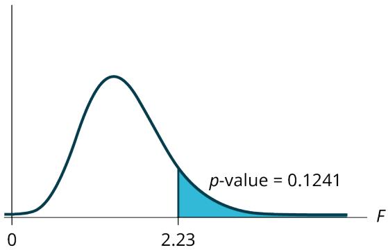
Figure 12.3.5 — The \(F_{3,16}\) curve with the test statistic marked.
area
| Metric | Value |
|---|---|
| p-value | 0.1241 |
Probability statement: p-value = \(P(F > 2.23) = 0.1241\)
Compare \(\alpha\) and the p-value: \(\alpha = 0.01\)
$$p\text{-value} = 0.1241$$\(\alpha <\) p-value
Make a decision: Since \(\alpha <\) p-value, you cannot reject \(H_0\).
Answer: There is not sufficient evidence to conclude that there is a difference among the mean grades for the sororities.

Figure 12.3.6 — TI-84 ANOVA output for the sorority data.
Using the TI-83, 83+, 84, 84+ Calculator
Put the data into lists \(L_1\), \(L_2\), \(L_3\), and \(L_4\). Press STAT and arrow over to TESTS. Arrow down to F:ANOVA. Press ENTER and enter (L1, L2, L3, L4).
The calculator displays the F statistic, the p-value and the values for the one-way ANOVA table:
F = 2.2303
p = 0.1241 (p-value)
Factor
df = 3
SS = 2.88732
MS = 0.96244
Error
df = 16
SS = 6.9044
MS = 0.431525

Figure 12.3.7 — Calculator keystrokes for the sorority ANOVA.
Notice how this example mirrors Example 12.3.1 step for step — only the significance level changed (1% instead of 5%) and the decision flipped. That's a good reminder that "reject" or "don't reject" depends on the bar you set before collecting data, not just on the data itself.
An ANOVA table is printed with one cell rubbed out:
| Source of Variation | SS | df | MS | F |
|---|---|---|---|---|
| Factor (Between) | 96 | 3 | ? | ? |
| Error (Within) | 320 | 40 | 8 | |
| Total | 416 | 43 |
a) Fill in \(MS_{\text{between}}\) and \(F\).
b) How many groups were compared, and how many observations were there in total?
Solution — every entry in the table is forced by the others
Step 1 — Mean square between. A mean square is always its sum of squares divided by its own degrees of freedom:
$$ MS_{\text{between}} = \frac{96}{3} = 32 $$Step 2 — The F statistic.
$$ F = \frac{MS_{\text{between}}}{MS_{\text{within}}} = \frac{32}{8} = 4 $$Step 3 — Recover the counts from the degrees of freedom. The numerator df is \(k - 1 = 3\), so \(k = 4\) groups. The denominator df is \(N - k = 40\), so \(N = 44\)... but check it against the Total row: total df is \(N - 1 = 43\), which also gives \(N = 44\). The two agree, which is the arithmetic check worth doing every time.
Answer: \(MS_{\text{between}} = 32\), \(F = 4\); 4 groups, 44 observations in total.
12.3.4 When Every Group Is the Same Size
A design in which every group has the same number of observations is called balanced. The test runs exactly as before; the arithmetic is just tidier, because each group contributes equally to the within-group estimate.
Another fourth grader also grew bean plants, but this time in a jelly-like mass. The heights were (in inches) 24, 28, 25, 30, and 32. Do a one-way ANOVA test on the four groups. Are the heights of the bean plants different? Use the same method as shown in Example 12.3.3.
Solution
Jelly group statistics: mean = \(\frac{24+28+25+30+32}{5} = 27.8\); variance = \(\frac{(24-27.8)^2+(28-27.8)^2+(25-27.8)^2+(30-27.8)^2+(32-27.8)^2}{4} = \frac{14.44+0.04+7.84+4.84+17.64}{4} = \frac{44.8}{4} = 11.2\)
Variance of the four group means (24.2, 25.4, 24.4, 27.8): mean = 25.45; \(s_{\overline{x}}^2 = \frac{(24.2-25.45)^2+(25.4-25.45)^2+(24.4-25.45)^2+(27.8-25.45)^2}{3} = \frac{1.5625+0.0025+1.1025+5.5225}{3} = \frac{8.19}{3} = 2.73\)
Pooled variance (mean of 11.7, 18.3, 16.3, 11.2) = \(\frac{57.5}{4} = 14.375\)
F ratio: \(F' = \frac{n \cdot s_{\overline{x}}^2}{s_{\text{pooled}}^2} = \frac{(5)(2.73)}{14.375} = \frac{13.65}{14.375} \approx 0.95\)
Degrees of freedom: numerator = 4 − 1 = 3; denominator = 20 − 4 = 16. Distribution: \(F_{3,16}\).
p-value: \(P(F > 0.95) \approx 0.438\).
Decision: Since p-value = 0.438 > \(\alpha = 0.03\), do not reject \(H_0\).
Conclusion: Even with the jelly-like mass added, the evidence is not sufficient to conclude that the mean heights of the bean plants differ across the four growing media.
From the class, create four groups of the same size as follows: men under 22, men at least 22, women under 22, women at least 22. Have each member of each group record the number of states in the United States they have visited. Run an ANOVA test to determine if the average number of states visited in the four groups are the same. Test at a 1% level of significance. Use one of the solution sheets in Appendix E Solution Sheets.
A fourth grade class is studying the environment. One of the assignments is to grow bean plants in different soils. Tommy chose to grow his bean plants in soil found outside his classroom mixed with dryer lint. Tara chose to grow her bean plants in potting soil bought at the local nursery. Nick chose to grow his bean plants in soil from his mother's garden. No chemicals were used on the plants, only water. They were grown inside the classroom next to a large window. Each child grew five plants. At the end of the growing period, each plant was measured, producing the data (in inches) in Table 12.3.7.
| Tommy's Plants | Tara's Plants | Nick's Plants |
|---|---|---|
| 24 | 25 | 23 |
| 21 | 31 | 27 |
| 23 | 23 | 22 |
| 30 | 20 | 30 |
| 23 | 28 | 20 |
Does it appear that the three media in which the bean plants were grown produce the same mean height? Test at a 3% level of significance.
Solution
This time, we will perform the calculations that lead to the \(F'\) statistic. Notice that each group has the same number of plants, so we will use the formula \(F' = \frac{n \cdot s_{\overline{X}}^2}{s_{\text{pooled}}^2}\).
Step 1 — Calculate the sample mean and sample variance of each group.
| Tommy's Plants | Tara's Plants | Nick's Plants | |
|---|---|---|---|
| Sample Mean | 24.2 | 25.4 | 24.4 |
| Sample Variance | 11.7 | 18.3 | 16.3 |
Step 2 — Calculate the variance of the three group means (calculate the variance of 24.2, 25.4, and 24.4). Variance of the group means = 0.413 = \(s_{\overline{x}}^2\)
Then \(MS_{between} = ns_{\overline{x}}^2 = (5)(0.413)\) where n = 5 is the sample size (number of plants each child grew).
Step 3 — Calculate the mean of the three sample variances (calculate the mean of 11.7, 18.3, and 16.3). Mean of the sample variances = 15.433 = \(s_{\text{pooled}}^2\)
Then \(MS_{within} = s_{\text{pooled}}^2 = 15.433\).
Step 4 — Compute the F ratio.
$$F = \frac{MS_{\text{between}}}{MS_{\text{within}}} = \frac{ns_{\overline{x}}^2}{s_{\text{pooled}}^2} = \frac{(5)(0.413)}{15.433} = 0.134$$Step 5 — Degrees of freedom.
The dfs for the numerator = the number of groups − 1 = 3 − 1 = 2.
The dfs for the denominator = the total number of samples − the number of groups = 15 − 3 = 12.
The distribution for the test is \(F_{2,12}\) and the F statistic is F = 0.134.
Step 6 — p-value and decision. The p-value is \(P(F > 0.134) = 0.8759\).
Decision: Since \(\alpha = 0.03\) and the p-value = 0.8759, do not reject \(H_0\). (Why? Because the p-value is far larger than \(\alpha\) — an F of 0.134 is well below 1, meaning the variation between soils is tiny compared to the natural plant-to-plant variation within each soil.)
Answer: With a 3% level of significance, from the sample data, the evidence is not sufficient to conclude that the mean heights of the bean plants are different.

Figure 12.3.8 — TI-84 Fcdf calculation for the bean plant p-value.
Using the TI-83, 83+, 84, 84+ Calculator
To calculate the p-value:
- Press
2nd DISTR - Arrow down to
Fcdf(and pressENTER. - Enter
0.134, E99, 2, 12) - Press
ENTER
The p-value is 0.8759.

Figure 12.3.9 — Calculator keystrokes for Fcdf.
Here's a fourth soil to add to the study. You now have everything you need: compute each group's mean and variance, find the variance of the group means, pool the variances, and assemble the F ratio just as in Example 12.3.3.
Problem Set 12.3
Problem 1. State the three properties of the F distribution that hold no matter what the degrees of freedom are.
Solution
Step 1 — Identify the properties that hold for every F curve: The section lists five facts; the ones that hold regardless of the degrees of freedom are the shape and range facts.
Step 2 — State the three: 1. The curve is not symmetrical — it is skewed to the right. 2. The F statistic is always greater than or equal to zero. 3. There is a different curve for each pair of degrees of freedom (this is what makes the dfs essential to identifying the distribution).
Answer: The three universal properties are: (1) the F curve is skewed to the right (not symmetrical), (2) \(F \geq 0\) always, and (3) there is a separate F curve for each set of degrees of freedom.
Problem 2. Why does the F distribution have a different curve for each pair of degrees of freedom? What two numbers identify a specific F curve?
Solution
Step 1 — Explain why a different curve exists for each df pair: The F statistic is a ratio of two mean squares, and each mean square depends on its own degrees of freedom. Changing either df changes how much variability that mean square estimates, so the whole shape of the ratio's distribution changes.
Step 2 — Name the two identifying numbers: A specific F curve is identified by the ordered pair \((df_{num}, df_{denom})\): the numerator degrees of freedom (groups − 1) and the denominator degrees of freedom (total observations − groups). Order matters — \(F_{3,20}\) and \(F_{20,3}\) are different curves.
Answer: Each pair of dfs changes the ratio of two mean squares' distribution, so every \((df_{num}, df_{denom})\) pair has its own curve; the two numbers are the numerator df and denominator df, written as subscripts in order.
Problem 3. As both degrees of freedom grow very large, what well-known distribution does the F curve come to resemble?
Solution
Step 1 — Recall fact 4 from the section: As both the numerator and denominator degrees of freedom get larger, the sharp right skew of the F curve flattens out.
Step 2 — Name the limiting distribution: With both dfs large, the curve becomes tall and humped, centered near 1, approximating the normal distribution. This is visible in Figure 12.3.1 with \(F_{100,100}\).
Answer: As both degrees of freedom grow very large, the F curve comes to resemble the normal distribution.
Problem 4. Can an F statistic ever be negative? Explain why or why not based on how it is constructed from mean squares.
Solution
Step 1 — Look at how F is constructed: The F statistic is
$$F = \frac{MS_{\text{between}}}{MS_{\text{within}}}$$where each mean square is a sum of squares divided by its degrees of freedom.
Step 2 — Check whether either part can be negative: Sums of squares are built from squared deviations, so every term is nonnegative, and dividing by positive degrees of freedom keeps them nonnegative. A ratio of two nonnegative quantities (with nonzero denominator) cannot be negative.
Answer: No. An F statistic can never be negative, because it is a ratio of two mean squares, and mean squares come from squared deviations, which are always ≥ 0. A negative F indicates an arithmetic error.
Problem 5. In a one-way ANOVA with \(k = 6\) groups and \(n = 30\) total observations, find \(df(num)\) and \(df(denom)\), and name the distribution used for the test.
Solution
Step 1 — Compute the numerator df: The numerator degrees of freedom equal the number of groups minus one:
$$df(num) = k - 1 = 6 - 1 = 5$$Step 2 — Compute the denominator df: The denominator degrees of freedom equal the total number of observations minus the number of groups:
$$df(denom) = n - k = 30 - 6 = 24$$Step 3 — Name the distribution: The test uses an F distribution with those two dfs.
Answer: \(df(num) = 5\), \(df(denom) = 24\); the test uses the \(F_{5,24}\) distribution.
Problem 6. A researcher runs a one-way ANOVA and reports \(F_{2,27} = 5.61\) with a p-value of 0.008. At a 5% significance level, state the decision and write a conclusion in plain language.
Solution
Step 1 — Compare α to the p-value: Here \(\alpha = 0.05\) and p-value = 0.008. Since
$$\text{p-value} = 0.008 < \alpha = 0.05,$$we reject \(H_0\).
Step 2 — Write the conclusion in plain language: Rejecting \(H_0\) means the data give sufficient evidence that at least one group mean differs from the others. In context: at the 5% significance level, there is strong evidence that the means of the groups being compared are not all equal — the differences among the group means are unlikely to be due to chance alone.
Answer: Decision: reject \(H_0\). Conclusion: At the 5% significance level, there is sufficient evidence that at least one of the group means differs from the rest.
Problem 7. In an ANOVA table, the Factor (Between) sum of squares is 450 with 3 degrees of freedom, and the Error (Within) sum of squares is 1,200 with 36 degrees of freedom. Compute \(MS_{between}\), \(MS_{within}\), and the F statistic.
Solution
Step 1 — Compute \(MS_{between}\): A mean square is its sum of squares divided by its own degrees of freedom:
$$MS_{between} = \frac{450}{3} = 150$$Step 2 — Compute \(MS_{within}\):
$$MS_{within} = \frac{1200}{36} = 33.33$$Step 3 — Compute the F statistic: Divide the between mean square by the within mean square:
$$F = \frac{MS_{between}}{MS_{within}} = \frac{150}{33.33} \approx 4.50$$Answer: \(MS_{between} = 150\), \(MS_{within} \approx 33.33\), and \(F \approx 4.50\).
Problem 8. An ANOVA comparing four teaching methods produces \(F = 0.87\) with a p-value of 0.46. Explain, without doing any new calculations, why the between-group variation must be small relative to the within-group variation.
Solution
Step 1 — Interpret what a small F means: The F statistic is the ratio
$$F = \frac{MS_{between}}{MS_{within}}.$$Here \(F = 0.87 < 1\), which forces the numerator to be smaller than the denominator:
$$MS_{between} = 0.87 \cdot MS_{within} < MS_{within}.$$Step 2 — Translate into variation language: Since the between-group mean square is smaller than the within-group mean square, the variation among the four teaching-method group means is small relative to the natural variation of students within each method. That is exactly why the p-value is large (0.46): the observed differences among group means look like ordinary chance variation.
Answer: Because \(F = \frac{MS_{between}}{MS_{within}} = 0.87 < 1\), we must have \(MS_{between} < MS_{within}\); the between-group variation is smaller than the within-group variation, so no new calculations are needed.
Problem 9. A study uses a balanced design with 4 groups of 8 observations each. Verify that \(df(num) = 3\) and \(df(denom) = 28\), and explain what "balanced" means here.
Solution
Step 1 — Verify the numerator df: With \(k = 4\) groups,
$$df(num) = k - 1 = 4 - 1 = 3. ✓$$Step 2 — Verify the denominator df: With 4 groups of 8 observations each, the total is \(n = 32\):
$$df(denom) = n - k = 32 - 4 = 28. ✓$$(Equivalently, total df = 31, minus 3 for the factor, leaves 28.)
Step 3 — Explain "balanced": A design is balanced when every group contains the same number of observations. Here each of the 4 groups has exactly 8 observations, so the design is balanced — this makes the arithmetic tidier because each group contributes equally to the pooled within-group estimate.
Answer: Verified: \(df(num) = 3\) and \(df(denom) = 28\). "Balanced" means all 4 groups have the same sample size (8 each).
Problem 10. Using the TI-83/84, describe the full sequence of keystrokes needed to run a one-way ANOVA on data stored in lists \(L_1\) through \(L_3\), and name the two outputs that let you make your decision.
Solution
Step 1 — Enter the data: Press STAT, then 1: EDIT, and type the three data sets into lists \(L_1\), \(L_2\), and \(L_3\).
Step 2 — Run ANOVA: Press STAT, arrow over to TESTS, arrow down to ANOVA (on some models F:ANOVA), press ENTER, then enter (L1, L2, L3) and press ENTER.
Step 3 — Read the decision-making outputs: The screen displays the F statistic and the p-value, along with the full ANOVA table (SS, df, MS for Factor and Error). The two outputs used for the decision are:
- the p-value: compare it to \(\alpha\) — if p-value ≤ \(\alpha\), reject \(H_0\);
- the F statistic: the test statistic corresponding to that p-value on the appropriate F curve.
Answer: Keystrokes: STAT → 1: EDIT (enter data in \(L_1, L_2, L_3\)) → STAT → TESTS → ANOVA → (L1, L2, L3) → ENTER. The two decision outputs are the F statistic and the p-value.
Problem 11. Using the TI-83/84 Fcdf command, write the exact entry you would use to find \(P(F > 2.15)\) for an \(F_{5,20}\) distribution, and state what each of the four arguments represents.
Solution
Step 1 — Write the entry: To find the area to the right of 2.15 under the \(F_{5,20}\) curve, use
Fcdf(2.15, E99, 5, 20)
(accessed via 2nd DISTR, arrow down to Fcdf().
Step 2 — Explain each argument: 1. 2.15 — the lower bound of the interval (the observed F value). 2. E99 (\(10^{99}\)) — the upper bound, standing in for infinity since the F distribution extends indefinitely to the right. 3. 5 — the numerator degrees of freedom. 4. 20 — the denominator degrees of freedom.
Answer: Enter Fcdf(2.15, E99, 5, 20); the arguments are the lower bound (2.15), the upper bound (E99 ≈ ∞), the numerator df (5), and the denominator df (20).
Problem 12. Name two other uses of the F distribution mentioned in this section besides testing equality of several means, and state which of them this chapter covers.
Solution
Step 1 — Recall fact 5 from the section: Besides testing equality of several means (one-way ANOVA), the F distribution has other uses listed in the text.
Step 2 — Name the two other uses: (1) comparing two variances, and (2) two-way Analysis of Variance (two-way ANOVA).
Step 3 — State which this chapter covers: Two-Way Analysis is explicitly noted as beyond the scope of this chapter, so the use covered here (besides one-way ANOVA itself) is comparing two variances.
Answer: The two other uses are comparing two variances and two-way Analysis of Variance; two-way ANOVA is beyond the scope of this chapter, so comparing two variances is the one covered.
Key Terms
F distribution — a right-skewed probability distribution used for ANOVA tests; there is a separate curve for each pair of degrees of freedom.
degrees of freedom (dfs) — the pair of numbers \((df_{num}, df_{denom})\) that identifies which F curve to use; numerator df = groups − 1, denominator df = total samples − groups.
balanced design — an experimental design in which every group has the same number of observations.
one-way ANOVA — a hypothesis test comparing the means of three or more groups using the F statistic.