12.4 Test of Two Variances
SLO 4
Demonstrate an understanding of, and ability to use, basic ideas of statistical processes, including hypothesis tests and confidence interval estimation.
SLO 5
Identify appropriate statistical techniques and use technology-based statistical analysis to describe, interpret, and communicate results.
Learning Objectives
By the end of this section, you will be able to:
- explain when an F test of two variances is appropriate and what assumptions it requires;
- compute the F ratio from two sample variances and identify its degrees of freedom;
- carry out a full hypothesis test for the equality of two population variances and state a conclusion in context;
- interpret how close the F statistic is to one as evidence for or against equal variances.
12.4.1 Why Compare Variances
Another use of the F distribution is testing two variances. So far in this chapter we have mostly compared averages — but sometimes the question isn't "are these groups different on average?" It's "are these groups different in spread?" That question comes up more often than you might expect:
- College administrators would like two professors grading exams to show the same variation in their grading. You don't want one instructor whose scores swing wildly while another's stay tight — students in different sections should face comparable grading.
- If a lid is to fit a container, the variation in the lid's diameter and the container's diameter should match. A lid that averages the right size but wobbles between too big and too small won't seal anything.
- A supermarket might care about the variability of check-out times for two checkers, not just their average speed. Predictable wait times are easier to staff for and easier to promise to customers.
In each case we're comparing how spread out two populations are, which means comparing their variances. The tool for this comparison is the F test of two variances, and it uses the same F distribution you met earlier in this chapter.
12.4.2 Assumptions and Cautions
To perform an F test of two variances, the following must be true:
Two checkers can both average four minutes per customer, yet one might take anywhere from 2 to 6 minutes while the other stays between 3 and 5. Same average, very different experience. Predictability — low variation — is often exactly what a business or a school wants to measure, and that's what this test delivers.
- The populations from which the two samples are drawn are normally distributed.
- The two populations are independent of each other.
Unlike most other tests in this book, the F test for equality of two variances is very sensitive to deviations from normality. If the two distributions are not normal, the test can give p-values that are too high or too low, in unpredictable ways. Many texts suggest that students not use this test at all, but in the interest of completeness we include it here.
Think of this test as a precision instrument that only works on a level surface. If your data aren't roughly bell-shaped, the p-value it reports can't be trusted — so always check for normality before believing the result.
Why does this test break so easily when the data aren't normal? Every hypothesis test builds its p-value on a model of what the test statistic looks like when the null hypothesis is true. For most tests in this book, that model holds up reasonably well even when the population is a little lopsided. The F ratio doesn't get that protection: squaring amplifies outliers, and the ratio of two squared quantities inherits every distortion. So a slightly skewed population can push the p-value far from where it should be — sometimes too high, sometimes too low, with no way to tell which. That unpredictability is exactly why some textbooks advise skipping this test entirely. We keep it because it appears in real software output and in later courses, but treat it as a tool with a narrow range of safe use.
12.4.3 The F Ratio
Suppose we sample randomly from two independent normal populations. Let \(\sigma_{1}^{2}\) and \(\sigma_{2}^{2}\) be the population variances and \(s_{1}^{2}\) and \(s_{2}^{2}\) be the sample variances. Let the sample sizes be \(n_{1}\) and \(n_{2}\). Since we are interested in comparing the two sample variances, we use the F ratio:
$$F = \frac {\left[ \frac {(s _ {1}) ^ {2}}{(\sigma_ {1}) ^ {2}} \right]}{\left[ \frac {(s _ {2}) ^ {2}}{(\sigma_ {2}) ^ {2}} \right]}$$\(F\) has the distribution \(F \sim F(n_{1} - 1, n_{2} - 1)\), where \(n_{1}-1\) is the degrees of freedom for the numerator and \(n_{2}-1\) is the degrees of freedom for the denominator.
Notice what each piece of this fraction is doing. Each sample variance gets divided by the population variance it estimates, so the top and bottom each measure "how far did our sample variance land from the truth?" Taking the ratio of those two measures tells us whether they landed at similar distances — which is what equal population variances would predict.
If the null hypothesis is \(\sigma_1^2 = \sigma_2^2\), then the F ratio becomes
$$F = \frac{\left[\frac{(s_1)^2}{(\sigma_1)^2}\right]}{\left[\frac{(s_2)^2}{(\sigma_2)^2}\right]} = \frac{(s_1)^2}{(s_2)^2}.$$Under the null hypothesis the two population variances are equal, so the \(\sigma^2\) terms cancel — just like dividing out a common factor. What's left is simply the ratio of the two sample variances, which we can actually compute from data.
The F ratio could also be \(\frac{(s_2)^2}{(s_1)^2}\). Which one we use depends on \(H_a\) and on which sample variance is larger.
For each claim, state \(H_0\) and \(H_a\), and say whether the test is left-tailed, right-tailed, or two-tailed.
a) A machinist claims machine A's fill volumes vary less than machine B's.
b) A teacher wants to know whether two sections' score variances differ at all, with no direction in mind.
c) A lab claims its new assay is more variable than the old one.
Solution — the alternative picks the tail, every time
a) \(H_0: \sigma_A^2 = \sigma_B^2\), \(H_a: \sigma_A^2 < \sigma_B^2\). Putting A's variance in the numerator to match the claim makes small values of F the evidence, so the test is left-tailed.
b) \(H_0: \sigma_1^2 = \sigma_2^2\), \(H_a: \sigma_1^2 \neq \sigma_2^2\). No direction is claimed, so the test is two-tailed and the p-value doubles one tail's area.
c) \(H_0: \sigma_{\text{new}}^2 = \sigma_{\text{old}}^2\), \(H_a: \sigma_{\text{new}}^2 > \sigma_{\text{old}}^2\). With the new assay on top, large F is the evidence, so the test is right-tailed.
Answer: a) left-tailed, b) two-tailed, c) right-tailed. Write \(H_a\) first and the tail follows from it — do not pick the tail by looking at which number happens to be bigger.
Suppose we sample from two independent normal populations and want to compare their variances. Show why the general F ratio collapses to a simple ratio of sample variances when the null hypothesis says the two population variances are equal.
Solution
Step 1 — Write the general form: The F ratio compares each sample variance to the population variance it estimates:
$$F = \frac {\left[ \frac {(s _ {1}) ^ {2}}{(\sigma_ {1}) ^ {2}} \right]}{\left[ \frac {(s _ {2}) ^ {2}}{(\sigma_ {2}) ^ {2}} \right]}$$Step 2 — Apply the null hypothesis: If \(H_0\) states \(\sigma_1^2 = \sigma_2^2\), then both population variances are the same number. Call it \(\sigma^2\).
Step 3 — Cancel: Substituting \(\sigma^2\) for both denominators gives
$$F = \frac {\left[ \frac {(s _ {1}) ^ {2}}{\sigma^2} \right]}{\left[ \frac {(s _ {2}) ^ {2}}{\sigma^2} \right]} = \frac {(s _ {1}) ^ {2}}{(s _ {2}) ^ {2}}.$$The unknown population variance cancels completely, leaving a statistic we can compute directly from the two samples.
Answer: Under \(H_0\), \(F = \dfrac{s_1^2}{s_2^2}\), distributed as \(F(n_1 - 1,\ n_2 - 1)\).
12.4.4 Reading the F Statistic
If the two populations have equal variances, then \(s_1^2\) and \(s_2^2\) are close in value and \(F = \frac{(s_1)^2}{(s_2)^2}\) is close to one. But if the two population variances are very different, \(s_1^2\) and \(s_2^2\) tend to be very different too. Choosing \(s_1^2\) as the larger sample variance causes the ratio \(\frac{(s_1)^2}{(s_2)^2}\) to be greater than one. If \(s_1^2\) and \(s_2^2\) are far apart, then \(F\) is a large number.
Therefore, if F is close to one, the evidence favors the null hypothesis (the two population variances are equal). But if F is much larger than one, the evidence is against the null hypothesis. A test of two variances may be left-, right-, or two-tailed.
For most test statistics you've met, zero was the "nothing going on" value. Here it's one: a ratio of 1 means the two sample variances match perfectly. The farther F drifts above 1, the louder the evidence that the spreads differ.
Which tail the test uses depends entirely on the alternative hypothesis. If \(H_a\) claims the first variance is smaller, the test is left-tailed. If \(H_a\) claims it is larger — or if we simply put the larger sample variance on top — the test is right-tailed. And if \(H_a\) only claims the variances differ without saying which way, the test is two-tailed. Before you compute anything, write down \(H_a\) and let it choose the tail for you.
Two college instructors are interested in whether there is any variation in the way they grade math exams. They each grade the same set of 30 exams. The first instructor's grades have a variance of 52.3. The second instructor's grades have a variance of 89.9. Test the claim that the first instructor's variance is smaller. (In most colleges, it is desirable for the variances of exam grades to be nearly the same among instructors.) The level of significance is 10%.
Solution
Step 1 — Set up the notation: Let 1 and 2 indicate the first and second instructor, respectively. Then \(n_1 = n_2 = 30\).
Step 2 — State the hypotheses: The claim is that the first instructor's variance is smaller, so:
$$H_0: \sigma_1^2 = \sigma_2^2 \quad \text{and} \quad H_a: \sigma_1^2 < \sigma_2^2$$Step 3 — Calculate the test statistic: By the null hypothesis (\(\sigma_1^2 = \sigma_2^2\)), the F statistic is:
$$F = \frac {\left[ \frac {(s _ {1}) ^ {2}}{(\sigma_ {1}) ^ {2}} \right]}{\left[ \frac {(s _ {2}) ^ {2}}{(\sigma_ {2}) ^ {2}} \right]} = \frac {(s _ {1}) ^ 2}{(s _ {2}) ^ 2} = \frac {52.3}{89.9} = 0.5818$$Step 4 — Identify the distribution: \(F_{29,29}\), where \(n_1 - 1 = 29\) and \(n_2 - 1 = 29\).
Step 5 — Draw the graph: This test is left-tailed, because \(H_a\) uses a "<" sign. Label and shade appropriately.
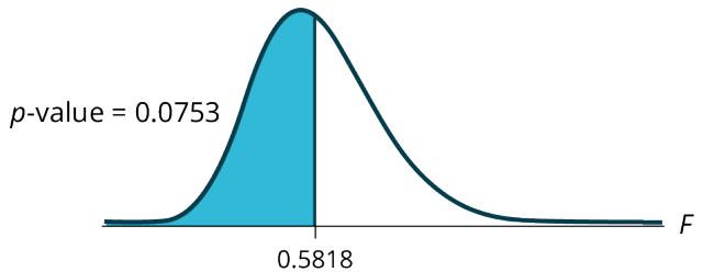
Figure 12.4.1 — Left-tailed F distribution with the rejection region shaded below F = 0.5818.
Step 6 — Probability statement: p-value = P(F < 0.5818) = 0.0753
Step 7 — Compare \(\alpha\) and the p-value: \(\alpha = 0.10\), and \(\alpha >\) p-value.
Step 8 — Make a decision: Since \(\alpha >\) p-value, reject \(H_0\).
Conclusion: With a 10% level of significance, from the data, there is sufficient evidence to conclude that the variance in grades for the first instructor is smaller.

Figure 12.4.2 — Calculator output confirming F = 0.5818 and p-value = 0.0753.
It's worth pausing on Step 3. Notice that here we did not put the larger variance on top — we put instructor 1's variance on top because the claim is about instructor 1 being smaller, and that made the test left-tailed. The choice of numerator follows the claim, not the size of the numbers. Had the claim been "instructor 2 varies less," we'd have flipped the fraction and run a right-tailed test instead.
12.4.5 Using the TI-83, 83+, 84, 84+ Calculator
Press STAT and arrow over to TESTS. Arrow down to D:2-SampFTest. Press ENTER. Arrow to Stats and press ENTER. For Sx1, n1, Sx2, and n2, enter \(\sqrt{52.3}\), 30, \(\sqrt{89.9}\), and 30. Press ENTER after each. Arrow to \(\sigma1\): and \(<\sigma2\). Press ENTER. Arrow down to Calculate and press ENTER. F = 0.5818 and p-value = 0.0753. Do the procedure again and try Draw instead of Calculate.

Figure 12.4.3 — The `Draw` output shades the left tail below F = 0.5818 and prints the same p-value.
Notice that the calculator asks for the sample standard deviations (Sx1, Sx2), not the variances — that's why we enter the square roots of 52.3 and 89.9. This trips up a lot of students: the problem hands you variances, the calculator wants standard deviations, and entering 52.3 directly produces a wrong F statistic with no error message. Always ask yourself which quantity you were given before typing anything in.
You are given two sample variances, \(s_1^2 = 40.96\) and \(s_2^2 = 21.16\), with \(n_1 = 16\) and \(n_2 = 16\).
a) Compute the F statistic with the larger variance on top, and give its degrees of freedom.
b) What four numbers would you type into the calculator's 2-SampFTest screen for Sx1, n1, Sx2, n2?
Solution — the calculator wants standard deviations
Step 1 — The F statistic.
$$ F = \frac{s_1^2}{s_2^2} = \frac{40.96}{21.16} \approx 1.9357 $$Step 2 — Degrees of freedom. \(df_{\text{num}} = n_1 - 1 = 15\) and \(df_{\text{denom}} = n_2 - 1 = 15\), so \(F \sim F_{15,15}\).
Step 3 — What the calculator screen wants. Sx1 and Sx2 are standard
deviations, not variances, so enter the square roots:
So you type 6.4, 16, 4.6, 16.
Step 4 — Why this matters. Typing 40.96 and 21.16 straight in produces an F of \((40.96/21.16)^2 \approx 3.75\) — a completely different statistic — and the calculator reports it without any complaint. The wrong answer looks exactly as trustworthy as the right one.
Answer: a) \(F \approx 1.9357\) on \(F_{15,15}\); b) 6.4, 16, 4.6, 16.
The New York Choral Society divides its male singers into four categories from highest voices to lowest: Tenor1, Tenor2, Bass1, Bass2. The table below gives the heights of the men in the Tenor1 and Bass2 groups. One suspects that taller men will have lower voices, and that the variance of height may go up with the lower voices as well. Do we have good evidence that the variance of the heights of singers in each of these two groups (Tenor1 and Bass2) are different?
| Tenor1 | Bass2 | Tenor1 | Bass2 |
|---|---|---|---|
| 69 | 72 | 70 | 68 |
| 72 | 75 | 68 | 75 |
| 71 | 67 | 64 | 68 |
| 66 | 75 | 73 | 70 |
| 76 | 74 | 66 | 72 |
| 74 | 72 | 68 | 67 |
| 71 | 72 | 67 | 70 |
| 66 | 74 | 64 | 70 |
| 68 | 72 | 69 | |
| 67 | 72 | 72 | |
| 70 | 74 | 71 | |
| 65 | 70 | 74 | |
| 72 | 66 | 75 |
Solution
Step 1 — Compute the sample statistics. From the data: Tenor1 has \(n_1 = 21\) heights with mean 68.90 inches and sample variance \(s_1^2 \approx 11.09\). Bass2 has \(n_2 = 26\) heights with mean 71.38 inches and sample variance \(s_2^2 \approx 7.45\).
Step 2 — State the hypotheses. We want evidence that the variances differ, so this is a two-tailed test:
$$H_0: \sigma_1^2 = \sigma_2^2 \quad \text{and} \quad H_a: \sigma_1^2 \neq \sigma_2^2$$Step 3 — Calculate the test statistic. Put the larger sample variance in the numerator:
$$F = \frac{s_1^2}{s_2^2} = \frac{11.09}{7.45} \approx 1.4894$$Step 4 — Identify the distribution: \(F_{20,25}\), since \(n_1 - 1 = 20\) and \(n_2 - 1 = 25\).
Step 5 — Find the p-value. This is a two-tailed test, so double the upper-tail area: p-value = 2 × P(F > 1.4894) ≈ 2(0.1715) ≈ 0.3430.
Step 6 — Make a decision. At any reasonable significance level (say \(\alpha = 0.05\)), the p-value is far larger than \(\alpha\), so we do not reject \(H_0\).
Conclusion: There is insufficient evidence to conclude that the variance of heights differs between the Tenor1 and Bass2 groups. The suspicion that height varies more among lower voices is not supported by these data.
Problem Set 12.4
Problem 1. State the two conditions that must hold before you run an F test of two variances, and explain in your own words why normality matters so much for this particular test.
Solution
Step 1 — State the two conditions: The F test of two variances requires that (1) the populations from which the two samples are drawn are normally distributed, and (2) the two populations are independent of each other.
Step 2 — Explain why normality matters here: Every hypothesis test builds its p-value on a model of what the test statistic looks like when \(H_0\) is true. Most tests in this book tolerate a little non-normality, but the F ratio does not: squaring amplifies outliers, and the ratio of two squared quantities inherits every distortion from the underlying distributions.
Step 3 — State the consequence: If the populations are not normal, the reported p-value can be too high or too low in unpredictable ways — there is no way to tell which direction the error goes. That unpredictability is why some textbooks advise not using this test at all unless normality is reasonably satisfied.
Answer: The conditions are (1) both populations are normally distributed and (2) the populations are independent. Normality matters because squaring amplifies outliers and the F ratio inherits every distortion, so with skewed data the p-value can be wrong in either direction, making the test's conclusion untrustworthy.
Problem 2. Two samples of sizes \(n_1 = 14\) and \(n_2 = 21\) are drawn from independent normal populations. What degrees of freedom identify the F distribution for the test of their variances?
Solution
Step 1 — Recall the degrees of freedom rule: For a test of two variances, the F statistic follows an F distribution with numerator degrees of freedom \(n_1 - 1\) (from sample 1) and denominator degrees of freedom \(n_2 - 1\) (from sample 2).
Step 2 — Compute each value: With \(n_1 = 14\):
$$n_1 - 1 = 14 - 1 = 13$$With \(n_2 = 21\):
$$n_2 - 1 = 21 - 1 = 20$$Answer: The test statistic follows an \(F_{13, 20}\) distribution — 13 degrees of freedom for the numerator and 20 for the denominator.
Problem 3. A sample from population 1 gives \(s_1^2 = 18.4\), and a sample from population 2 gives \(s_2^2 = 19.6\). Compute the F ratio and comment on whether it favors \(H_0\) or \(H_a\).
Solution
Step 1 — Compute the F ratio: Under \(H_0\), the F statistic is the ratio of the two sample variances:
$$F = \frac{s_1^2}{s_2^2} = \frac{18.4}{19.6} \approx 0.9388$$Step 2 — Interpret the value: The neutral value for this statistic is one, since a ratio of 1 means the two sample variances match exactly. Here \(F \approx 0.94\) is very close to one.
Step 3 — Draw the conclusion about evidence: Because the two sample variances are nearly equal, the data look exactly like what equal population variances would produce. This favors \(H_0\) (the variances are equal) rather than \(H_a\) (they differ).
Answer: \(F = \dfrac{18.4}{19.6} \approx 0.9388\). Since this is close to one, the data favor \(H_0\) — there is no sign of a difference in the two population variances.
Problem 4. A sample from population 1 gives \(s_1^2 = 45.0\), and a sample from population 2 gives \(s_2^2 = 5.0\). Compute the F ratio using the larger variance in the numerator, and state what a large value like this suggests about the two population variances.
Solution
Step 1 — Put the larger variance on top: Since \(s_1^2 = 45.0 > s_2^2 = 5.0\), we use:
$$F = \frac{s_1^2}{s_2^2} = \frac{45.0}{5.0} = 9.0$$Step 2 — Interpret the large value: A value of one would mean the sample variances agree perfectly; values far above one mean they are far apart. Here the first sample's variance is nine times the second's.
Step 3 — State what this suggests: An F ratio as large as 9 suggests the two population variances are quite different — specifically, it suggests \(\sigma_1^2\) is substantially larger than \(\sigma_2^2\). Such a large value constitutes strong evidence against \(H_0: \sigma_1^2 = \sigma_2^2\) (a formal decision would still require comparing the p-value to \(\alpha\)).
Answer: \(F = 9.0\). A value this far above one strongly suggests the two population variances are unequal, with population 1 having much greater spread than population 2.
Problem 5. Explain why the F ratio reduces to \(\frac{s_1^2}{s_2^2}\) when the null hypothesis is true, and why that reduction is what makes the test usable at all.
Solution
Step 1 — Start from the general F ratio: The general form divides each sample variance by the population variance it estimates:
$$F = \frac {\left[ \frac {(s _ {1}) ^ {2}}{(\sigma_ {1}) ^ {2}} \right]}{\left[ \frac {(s _ {2}) ^ {2}}{(\sigma_ {2}) ^ {2}} \right]}$$Step 2 — Apply the null hypothesis: When \(H_0\) is true, \(\sigma_1^2 = \sigma_2^2\). Both unknown population variances are then the same number, so call them both \(\sigma^2\).
Step 3 — Cancel the common factor: Substituting gives
$$F = \frac {\left[ \frac {(s _ {1}) ^ {2}}{\sigma^2} \right]}{\left[ \frac {(s _ {2}) ^ {2}}{\sigma^2} \right]} = \frac {(s _ {1}) ^ {2}}{(s _ {2}) ^ {2}}.$$The unknown \(\sigma^2\) cancels just like any common factor in a fraction.
Step 4 — Explain why this makes the test usable: Before canceling, the formula contains \(\sigma_1^2\) and \(\sigma_2^2\) — quantities we never know (if we knew them, we wouldn't need to test anything). After canceling, only \(s_1^2\) and \(s_2^2\) remain, and those we compute directly from data. The cancellation under \(H_0\) is precisely what turns an uncomputable expression into a usable test statistic.
Answer: Under \(H_0\), both population variances are equal, so the common \(\sigma^2\) cancels, leaving \(F = \dfrac{s_1^2}{s_2^2}\). This reduction removes the unknown parameters and leaves only computable sample quantities — without it, no test would be possible.
Problem 6. An instructor claims her exam-score variance is smaller than a colleague's. She has \(n_1 = 25\) scores with variance 31.2; the colleague has \(n_2 = 25\) scores with variance 58.7. State \(H_0\) and \(H_a\), decide the tail of the test, and explain your reasoning.
Solution
Step 1 — Identify the claim: The claim is that her exam-score variance is smaller than the colleague's, so instructor 1's variance goes in the comparison as the smaller quantity.
Step 2 — Write the hypotheses:
$$H_0: \sigma_1^2 = \sigma_2^2 \quad \text{and} \quad H_a: \sigma_1^2 < \sigma_2^2$$The null always asserts equality (no difference); the alternative carries the claim.
Step 3 — Decide the tail: Because \(H_a\) uses a "<" sign — small values of the F ratio support the claim that \(\sigma_1^2 < \sigma_2^2\) — the test is left-tailed.
Step 4 — Explain the reasoning: The tail is chosen entirely by the alternative hypothesis, not by which sample variance happens to be larger. Here the claim puts instructor 1's variance on top of the fraction, so evidence in her favor appears as a small F value, i.e., area in the left tail of the F distribution.
Answer: \(H_0: \sigma_1^2 = \sigma_2^2\), \(H_a: \sigma_1^2 < \sigma_2^2\); the test is left-tailed because the alternative claims the first variance is smaller, making small F values the supporting evidence.
Problem 7. For the setup in Problem 12.4.6, compute the F statistic and give the degrees of freedom for its distribution.
Solution
Step 1 — Compute the F statistic: Following Problem 12.4.6, instructor 1's variance goes in the numerator to match the claim:
$$F = \frac{s_1^2}{s_2^2} = \frac{31.2}{58.7} \approx 0.5315$$Step 2 — Find the degrees of freedom: Numerator: \(n_1 - 1 = 25 - 1 = 24\). Denominator: \(n_2 - 1 = 25 - 1 = 24\).
Step 3 — State the distribution: The test statistic follows \(F \sim F(24, 24)\).
Answer: \(F = \dfrac{31.2}{58.7} \approx 0.5315\), distributed as \(F_{24, 24}\).
Problem 8. A quality engineer wants to know whether two filling machines produce fills with equal variability. Machine A: \(n = 20\), variance 0.81. Machine B: \(n = 24\), variance 0.79. Without computing a p-value, explain what the F ratio tells you here and why no formal conclusion needs a table lookup.
Solution
Step 1 — Compute the F ratio: Putting machine A's variance on top:
$$F = \frac{s_A^2}{s_B^2} = \frac{0.81}{0.79} \approx 1.0253$$Step 2 — Interpret the value: One is the neutral value for an F ratio — it means the two sample variances agree perfectly. Here \(F \approx 1.03\) is extremely close to one: the machines' fill variabilities differ by only about 2.5%.
Step 3 — Explain why no table lookup is needed: Evidence against \(H_0\) comes from F drifting far from one. A statistic essentially equal to one lies near the center of the null distribution, where almost all of the probability mass sits when the variances truly are equal. The p-value would be close to its maximum possible size (near 1 for a two-tailed test), far above any conventional significance level, so rejection is impossible regardless of the exact cutoff.
Answer: \(F = \dfrac{0.81}{0.79} \approx 1.0253\). Because the ratio is nearly one, the data look exactly like what equal variances predicts; the p-value would be very large, so no formal lookup is needed to conclude there is no evidence of a difference in variability between the two filling machines.
Problem 9. Why does the calculator's D:2-SampFTest ask for Sx1 and Sx2 rather than the variances, and what must you do to the variances 52.3 and 89.9 before entering them?
Solution
Step 1 — Explain why the calculator asks for standard deviations: The D:2-SampFTest routine is built around the same machinery as the two-sample t procedures, whose inputs Sx1 and Sx2 are sample standard deviations. Internally the calculator squares these values to get the variances it needs for the F ratio, so the input convention matches the rest of the STAT TESTS menu rather than the variance-based formula in the textbook.
Step 2 — Convert before entering: The problem supplies variances, so take square roots first:
$$\sqrt{52.3} \approx 7.2319 \qquad \sqrt{89.9} \approx 9.4816$$Step 3 — Note the danger of skipping this step: Entering 52.3 and 89.9 directly makes the calculator treat them as standard deviations, squaring them into variances of about 2735 and 8082. The resulting F statistic is completely wrong, yet the calculator reports it without any error message — the wrong answer looks exactly as trustworthy as the right one.
Answer: The calculator expects standard deviations because Sx1/Sx2 follow the menu-wide convention and it squares them internally. You must enter \(\sqrt{52.3} \approx 7.2319\) and \(\sqrt{89.9} \approx 9.4816\), not the variances themselves.
Problem 10. A student runs an F test on two clearly skewed data sets and reports a p-value of 0.02. Explain, using the sensitivity discussion in this section, why that p-value may not mean what the student thinks it means.
Solution
Step 1 — Recall what the p-value model assumes: A p-value is computed under a model of how the test statistic behaves when \(H_0\) is true. For the F test, that model assumes both populations are normally distributed.
Step 2 — Apply the sensitivity discussion: The F ratio is unusually fragile to violations of this assumption. Squaring amplifies outliers, and the ratio of two squared quantities inherits every distortion from the underlying distributions. With clearly skewed data, the actual distribution of the F statistic under \(H_0\) can be very different from the theoretical F distribution the p-value was read from.
Step 3 — Explain the consequence for the student's result: Because the skew distorts the null distribution in unpredictable ways — sometimes pushing p-values too high, sometimes too low, with no way to tell which — the reported p-value of 0.02 may be far from the true probability of seeing data this extreme if the variances were equal. It could correspond to a true p-value well above 0.05 (in which case the "significant" finding is spurious) or even further below it. Either way, the number cannot be taken at face value.
Answer: The p-value of 0.02 rests on the normality assumption, and the F test is notoriously sensitive to its violation: with clearly skewed data, the true null distribution of F may differ greatly from the theoretical one, so the reported p-value may be too high or too low by an unknowable amount. The student should check normality (or use a more robust procedure) before trusting that result.
Problem 11. Give one real-world scenario (different from the three in this section) where comparing two variances is the natural question, and state what unequal variances would mean practically in your scenario.
Solution
Step 1 — Give a scenario: Consider two pharmacies filling prescriptions. Management wants to know whether the two pharmacies' waiting times have the same variability — not whether their average waits are equal.
Step 2 — State why variances are the natural question: Two pharmacies could both average 15 minutes per prescription, but if one's wait swings between 5 and 30 minutes while the other stays between 12 and 18, customers experience them very differently. Predictability is what matters for staffing and for service guarantees, and predictability is measured by variance.
Step 3 — Interpret unequal variances practically: If the test showed pharmacy A's wait-time variance significantly larger than pharmacy B's, it would mean A's service is unreliable even if its average looks fine: customers at A face unpredictable waits, so management might shift staff toward A, investigate its workflow, or quote wider time windows to A's customers. Equal variances would mean both locations deliver equally dependable service.
Answer: Example: comparing the variability of customer waiting times at two pharmacies. Unequal variances would mean one location's waits are far less predictable than the other's — a practical reliability problem even if the average waits match — while equal variances would indicate both provide equally dependable service.
Problem 12. True or false, and justify: "An F statistic very close to one is strong evidence for the alternative hypothesis."
Solution
Step 1 — Evaluate the statement: The statement is false — in fact it has things backwards.
Step 2 — Explain why: One is the neutral value of the F ratio: if the two population variances really are equal, the sample variances tend to be close together and F lands near one. So an F statistic very close to one is exactly what the null hypothesis predicts.
Step 3 — State the correct reading: Evidence against \(H_0\) comes from F drifting far from one — typically far above one when the larger variance is placed in the numerator. An F near one therefore supports the null hypothesis (equal variances), not the alternative.
Answer: False. An F statistic close to one means the two sample variances nearly match, which is precisely what equal population variances would produce — so it is strong evidence for the null hypothesis, not for the alternative.
Key Terms
F ratio — the test statistic for comparing two variances; under the null hypothesis it reduces to the ratio of the two sample variances, \(\frac{s_1^2}{s_2^2}\).
degrees of freedom (numerator/denominator) — the values \(n_1 - 1\) and \(n_2 - 1\) that identify which F distribution the test statistic follows.
test of two variances — a hypothesis test using the F distribution to decide whether two independent, normally distributed populations have equal variances.