2.7 Measures of the Spread of the Data
SLO 2
Identify appropriate graphs and summary statistics for variables and relationships between them and correctly interpret information from graphs and summary statistics.
The standard deviation is the summary statistic for spread, the piece the center and the shape leave out. You learn to compute it, to read any value as so many standard deviations from its mean, and to use that z-score to compare numbers from two data sets that share no scale.
Learning Objectives
By the end of this section, you will be able to:
- explain what the standard deviation measures and why a larger value means the data are more spread out;
- calculate the sample and population standard deviation from a data list and from a grouped frequency table;
- express any data value as the mean plus a number of standard deviations, and convert that count into a z-score;
- compare values that come from two different data sets by putting them on the same z-score scale;
- state what fraction of the data falls within two or three standard deviations of the mean, for any distribution and for a bell-shaped one.
Sections 2.5 and 2.6 gave you numbers for the center of a data set and a way to read its shape. Both leave out something a reader needs. Two classes can have the same average score of 75 and look nothing alike: one where almost everybody scored between 72 and 78, and one where half the class scored in the 50s and half in the 90s. The center is identical. The experience of being in those two rooms is not.
What separates them is variation, also called spread — how far the data values sit from their mean. This section gives you the standard tool for measuring it, the standard deviation, and then the trick that makes it genuinely useful: once you know a data set's mean and standard deviation, you can say whether any particular value is ordinary or unusual, and you can compare values pulled from two completely different data sets.
2.7.1 What the Standard Deviation Tells You
The standard deviation is a number that measures how far the data values are from their mean. It is always positive or zero. It is small when the data are concentrated close to the mean, and larger when the data values are spread out from the mean.
Measure how far every value sits from the mean, then ask what a typical one of those distances is. That is the standard deviation, in the same units as the data. Minutes of waiting produce a standard deviation in minutes.
The standard deviation does two jobs at once. It gives you a single number for the overall amount of variation in a data set, and it gives you a yardstick for deciding whether one particular data value is close to or far from the mean.
Start with the first job. Suppose we are studying how long customers wait in line at the checkout of two supermarkets. Call them Supermarket A and Supermarket B. The average wait at both is five minutes. At Supermarket A the standard deviation of the wait time is two minutes; at Supermarket B it is four minutes.
Because Supermarket B has the higher standard deviation, we know there is more variation in its wait times. Overall, waits at Supermarket B are more spread out from the average, and waits at Supermarket A are more concentrated near the average. If you value predictability — knowing roughly how long the errand will take — Supermarket A is the better line to stand in, even though the two averages are identical.
Now the second job. Rosa and Binh both shop at Supermarket A, where the mean wait is five minutes and the standard deviation is two minutes. Rosa waits at the checkout for seven minutes and Binh waits for one minute.
Rosa's wait of seven minutes is two minutes longer than the average of five. Two minutes is exactly one standard deviation, so Rosa's wait is one standard deviation above the mean.
Binh's wait of one minute is four minutes less than the average of five. Four minutes is two standard deviations, so Binh's wait is two standard deviations below the mean.
That second number is the interesting one. A data value two standard deviations from the mean sits on the borderline of what many statisticians would call far from the mean. Treat the two-standard-deviation line as an approximate rule of thumb rather than a rigid rule — the shape of the distribution affects how much of the data lands beyond it, which is something Section 2.6 already hinted at and later chapters make precise.
A number line makes the counting concrete. Put five and seven on a number line: seven is to the right of five, one standard deviation to the right, because \(5 + (1)(2) = 7\). If one were also part of the data set, one is two standard deviations to the left of five, because \(5 + (-2)(2) = 1\).
Figure 2.7.1 — Counting standard deviations along a number line: from a mean of five, one step of two minutes to the right lands on seven, and two steps to the left land on one.
That counting generalizes into the single most useful equation in this section:
$$\text{value} = \text{mean} + (\#\text{ofSTDEVs})(\text{standard deviation})$$Here \(\#\text{ofSTDEVs}\) is the number of standard deviations, and it does not have to be a whole number. A value 1.5 standard deviations above the mean is a perfectly ordinary thing to talk about.
The equation comes in two flavors, depending on whether the numbers describe a sample or a whole population:
$$\text{sample:}\quad x = \bar{x} + (\#\text{ofSTDEVs})(s) \qquad \text{population:}\quad x = \mu + (\#\text{ofSTDEVs})(\sigma)$$The lower-case letter \(s\) stands for the sample standard deviation and the Greek letter \(\sigma\) (sigma, lower case) stands for the population standard deviation. Likewise \(\bar{x}\) is the sample mean and \(\mu\) is the population mean. Same idea, different alphabet, and which alphabet you use tells the reader whether you measured everybody or only a sample.
A bus route has a mean travel time of 24 minutes with a standard deviation of 3 minutes. Cruz Delgado rides it every morning, and their trip today took 33 minutes.
a. How many standard deviations above the mean was Cruz's trip?
b. What travel time would be two standard deviations below the mean?
Solution
Step 1 — Find the distance from the mean (part a). Their trip was \(33 - 24 = 9\) minutes longer than average.
Step 2 — Convert minutes into standard deviations. One standard deviation is 3 minutes, so 9 minutes is
$$\frac{9}{3} = 3 \text{ standard deviations.}$$Step 3 — Use the equation in the other direction (part b). Two standard deviations below the mean means \(\#\text{ofSTDEVs} = -2\):
$$\text{value} = 24 + (-2)(3) = 18 \text{ minutes.}$$Answer: Cruz's trip was three standard deviations above the mean, which is unusually long — well past the two-standard-deviation rule of thumb. A trip two standard deviations below the mean would take 18 minutes.
2.7.2 Calculating the Standard Deviation
To build a standard deviation you first need the distance from each value to the mean. If \(x\) is a data value, the difference \(x - \text{mean}\) is called its deviation. For population data the deviation is \(x - \mu\); for sample data it is \(x - \bar{x}\). A data set has as many deviations as it has values.
The procedure for turning deviations into a standard deviation depends on whether the numbers are the entire population or a sample. The calculations are similar but not identical, which is why the two cases get different symbols. If the sample has the same characteristics as the population, then \(s\) should be a good estimate of \(\sigma\).
To get to the standard deviation we go through the variance first.
Definition 2.7.2 — A deviation is a signed distance to the mean, and the signed distances always cancel to zero.
The variance is the average of the squares of the deviations. The symbol \(\sigma^2\) represents the population variance and \(s^2\) represents the sample variance. The standard deviation is the square root of the variance: \(\sigma = \sqrt{\sigma^2}\) and \(s = \sqrt{s^2}\).
Add the raw deviations and you always get zero — the positives and negatives cancel exactly, which is what "balance point" means. Squaring makes every term positive so the total measures size instead of cancelling itself out.
Squaring solves the cancellation problem but creates a units problem: squared minutes are not minutes. Taking the square root at the end undoes the squaring and returns the answer to the same units as the data. So you can think of the standard deviation as a special kind of average of the deviations.
The one remaining choice is what to divide by. If the numbers come from a census of the entire population, divide by \(N\), the number of items in the population. If the data are a sample, divide by \(n - 1\), one less than the number of items in the sample.
For the sample standard deviation the denominator is \(n - 1\), the sample size MINUS 1.
For the population standard deviation the denominator is \(N\), the number of items in the population.
In both pairs, \(f\) represents the frequency with which a value appears. If a value appears once, \(f\) is one; if it appears three times, \(f\) is three. The second formula in each pair is the shortcut you use when the data arrive as a frequency table instead of a long list.
Definition 2.7.3 — Squaring each deviation turns signed numbers that cancel into positive areas that cannot.
How much a statistic varies from one sample to another is the sampling variability of a statistic.
Definition 2.7.4 — Three samples from one unchanged population give three different means; that spread is the sampling variability.
The standard error of the mean is the standard deviation of the sampling distribution of the mean, written \(\dfrac{\sigma}{\sqrt{n}}\), where \(\sigma\) is the population standard deviation and \(n\) is the sample size. It is the usual way to measure the sampling variability of a sample mean.
In practice you compute a standard deviation with a calculator or software, not by hand. What matters is choosing the right one: on a TI-83/84 the summary statistics list both \(\sigma_x\) and \(s_x\), and picking the population value for sample data is a real mistake, not a rounding difference.
The standard error is the tool for a different question — not "how spread out is this data?" but "how much would my answer wobble if I drew a different sample?" It comes back in force in the chapter on the Central Limit Theorem; here it is enough to know the name and the notation.
The worked example below does the arithmetic the long way anyway, because seeing the table built column by column is what makes the formula stop looking arbitrary. Every quantity in it is something you have already met: a list of values, how often each one occurs, and how far each one sits from the mean. The only new move is squaring the deviations before averaging them. Read it once for the mechanics, then trust your calculator for the rest of your life. The calculator instructions appear at the end of the example.
Ryan Whitfield keeps the roster for a baseball team, and he recorded the ages of the players:
21; 21; 22; 23; 24; 24; 25; 25; 28; 29; 29; 31; 32; 33; 33; 34; 35; 36; 36; 36; 36; 38; 38; 38; 40
Use your calculator or computer to find the mean and standard deviation. Then find the value that is two standard deviations above the mean.
Solution
Step 1 — The mean. There are 25 ages and they total 767, so
$$\bar{x} = \frac{767}{25} = 30.68 \text{ years.}$$Step 2 — The standard deviation. Entering the list and reading \(Sx\) from 1-VarStats gives
Step 3 — Two standard deviations above the mean.
$$\bar{x} + 2s = 30.68 + (2)(6.09) = 42.86$$Answer: The mean age is 30.68 years with a standard deviation of about 6.09 years. Two standard deviations above the mean is about 42.9 years — older than every player on the roster, which tells you nobody on this team is unusually old for it.
In a fifth grade class, the teacher, Ms. Nia Coleman, was interested in the average age and the sample standard deviation of the ages of her students. The following data are the ages for a SAMPLE of \(n = 20\) fifth grade students, rounded to the nearest half year:
9; 9.5; 9.5; 10; 10; 10; 10; 10.5; 10.5; 10.5; 10.5; 11; 11; 11; 11; 11; 11; 11.5; 11.5; 11.5
Recall that \(\text{value} = \text{mean} + (\#\text{ofSTDEVs})(\text{standard deviation})\). Because the data are from a sample, use \(x = \bar{x} + (\#\text{ofSTDEVs})(s)\).
a. Verify the mean and standard deviation on your calculator or computer.
b. Find the value that is one standard deviation above the mean, \((\bar{x} + 1s)\).
c. Find the value that is two standard deviations below the mean, \((\bar{x} - 2s)\).
d. Find the values that are 1.5 standard deviations below and above the mean.
Solution
Step 1 — The mean. Group the repeated values and divide by 20:
$$\bar{x} = \frac{9 + 9.5(2) + 10(4) + 10.5(4) + 11(6) + 11.5(3)}{20}$$ $$= \frac{210.5}{20} = 10.525$$The average age is 10.53 years, rounded to two places.
Step 2 — The variance, built in a table. Each row takes one distinct age, records how often it occurs, subtracts the mean to get the deviation, squares that deviation, and multiplies by the frequency.
| Data \(x\) | Freq. \(f\) | Deviation \((x - \bar{x})\) | \((x - \bar{x})^2\) | \(f(x - \bar{x})^2\) |
|---|---|---|---|---|
| 9 | 1 | 9 - 10.525 = -1.525 | 2.325625 | 2.325625 |
| 9.5 | 2 | 9.5 - 10.525 = -1.025 | 1.050625 | 2.101250 |
| 10 | 4 | 10 - 10.525 = -0.525 | 0.275625 | 1.102500 |
| 10.5 | 4 | 10.5 - 10.525 = -0.025 | 0.000625 | 0.002500 |
| 11 | 6 | 11 - 10.525 = 0.475 | 0.225625 | 1.353750 |
| 11.5 | 3 | 11.5 - 10.525 = 0.975 | 0.950625 | 2.851875 |
| Total | 20 | 9.7375 |
The sample variance is the sum of the last column divided by one less than the number of data values:
$$s^2 = \frac{9.7375}{20 - 1} = 0.5125$$Step 3 — The standard deviation (part a). Take the square root:
$$s = \sqrt{0.5125} = 0.715891 \approx 0.72$$So \(\bar{x} = 10.53\) and \(s = 0.72\). On a calculator you get the same two numbers directly, and because it does not round the intermediate results its answer is the more accurate one.
Step 4 — One standard deviation above the mean (part b).
$$\bar{x} + 1s = 10.53 + (1)(0.72) = 11.25$$Step 5 — Two standard deviations below the mean (part c).
$$\bar{x} - 2s = 10.53 - (2)(0.72) = 9.09$$Step 6 — One and a half standard deviations either way (part d).
$$\bar{x} - 1.5s = 10.53 - (1.5)(0.72) = 9.45 \qquad \bar{x} + 1.5s = 10.53 + (1.5)(0.72) = 11.61$$Answer: \(\bar{x} = 10.53\) years and \(s = 0.72\) years. One standard deviation above the mean is 11.25 years; two below is 9.09 years; 1.5 standard deviations either side gives 9.45 and 11.61 years.
Doing part a on a TI-83, 83+, 84, or 84+. Clear lists L1 and L2 with STAT 4:ClrList, entering 2nd 1 for L1, a comma, then 2nd 2 for L2. Open the list editor with STAT 1:EDIT, clearing any old lists by arrowing up onto the name, pressing CLEAR, and arrowing back down. Put the six distinct data values (9, 9.5, 10, 10.5, 11, 11.5) into L1 and their frequencies (1, 2, 4, 4, 6, 3) into L2. Press STAT, arrow to CALC, choose 1:1-VarStats, and enter L1 (2nd 1), a comma, L2 (2nd 2) — the comma matters. Press ENTER. The screen reports \(\bar{x} = 10.525\), and you read \(Sx = 0.715891\) because this is sample data, not a population.
Try it in rāSHio
Open rāSHio, paste the twenty ages into File → Delimited List…, then choose Stats → Summary Statistics. The mean and the standard deviation come back in the same panel, and the panel labels which standard deviation is which — so the one real trap in this calculation, reading the population value for sample data, is a label you can see rather than a menu entry you have to remember.
Figure 2.7.2 — Reading the mean and the standard deviation off one panel in rāSHio: Stats → Summary Statistics.
Why the Deviations Get Squared and Divided by n Minus 1
The deviation column is where the meaning lives. It shows how spread out the data are about the mean. The value 11.5 is farther from the mean than 11 is, and the deviations say so: 0.975 against 0.475. A positive deviation means the data value is above the mean; a negative deviation means it is below. The deviation for the age nine is \(-1.525\).
Add all twenty deviations and the sum is exactly zero, every time, for every data set. That is why you cannot simply add deviations to measure spread — the answer would always be nothing. Squaring makes each one positive, so the total finally reflects how far the values actually are from the mean, and the variance is that average squared deviation.
The variance is a squared measure, so it does not carry the units of the data. Taking the square root fixes this, and the standard deviation measures the spread in the same units as the data.
Notice too that the division was by \(n - 1 = 19\), not by 20, because the data are a sample. Why not divide by \(n\)? Because the sample variance is an estimate of the population variance, and the mathematics behind these calculations shows that dividing by \(n - 1\) gives a better estimate.
A standard deviation of zero is not an error — it means every value in the set is identical, so nothing deviates from anything. From there, the more the values disagree with each other, the larger \(s\) or \(\sigma\) grows, and a single outlier can make it very large.
Keep your attention on what the standard deviation tells you about the data rather than on the arithmetic. Describing data with reference to spread is called variability, and the variability you observe depends on how the outcomes were obtained — by measuring, by random sampling, or otherwise.
The standard deviation can seem unclear when it is first presented, and graphing your data is the cure. In symmetrical distributions it is very helpful. In skewed distributions it may not help much, because the two sides of a skewed distribution have different spreads and one number cannot describe both. For a skewed distribution you are better off looking at the first quartile, the median, the third quartile, the smallest value, and the largest value. Numbers alone can mislead, so always graph your data — a histogram or a box plot — before you decide what the numbers mean. The next example does exactly that, putting both graphs on one set of axes so you can see the same spread twice.
Mateo Herrera surveyed the pet stores near him and recorded how many different types of pet food each one carries.
6; 6; 6; 6; 7; 7; 7; 7; 7; 8; 9; 9; 9; 9; 10; 10; 10; 10; 10; 11; 11; 11; 11; 12; 12; 12; 12; 12; 12
Calculate the sample mean and the sample standard deviation to one decimal place using a TI-83+ or TI-84 calculator.
Solution
Step 1 — Set up the lists. There are 29 values. Enter the seven distinct counts into L1 and their frequencies into L2: 6 appears 4 times, 7 appears 5 times, 8 once, 9 four times, 10 five times, 11 four times, and 12 six times.
Step 2 — The mean. The 29 values total 269, so
$$\bar{x} = \frac{269}{29} \approx 9.3 \text{ types.}$$Step 3 — The standard deviation. Reading \(Sx\) from 1-VarStats gives
Answer: The sample mean is about 9.3 types of pet food and the sample standard deviation is about 2.2 types. A store carrying 5 types would be just under two standard deviations below the mean, which is close to the borderline for unusual.
A class of 31 students took an exam. The scores were
33; 42; 49; 49; 53; 55; 55; 61; 63; 67; 68; 68; 69; 69; 72; 73; 74; 78; 80; 83; 88; 88; 88; 90; 92; 94; 94; 94; 94; 96; 100
a. Create a chart containing the data, frequencies, relative frequencies, and cumulative relative frequencies to three decimal places.
b. Calculate the following to one decimal place using a TI-83+ or TI-84 calculator: the sample mean, the sample standard deviation, the median, the first quartile, the third quartile, and the IQR.
c. Construct a box plot and a histogram on the same set of axes. Make comments about the box plot, the histogram, and the chart.
Solution
Step 1 — The chart (part a). Each score's relative frequency is its frequency divided by 31, and the cumulative column running total.
| Data | Frequency | Relative Frequency | Cumulative Relative Frequency |
|---|---|---|---|
| 33 | 1 | 0.032 | 0.032 |
| 42 | 1 | 0.032 | 0.064 |
| 49 | 2 | 0.065 | 0.129 |
| 53 | 1 | 0.032 | 0.161 |
| 55 | 2 | 0.065 | 0.226 |
| 61 | 1 | 0.032 | 0.258 |
| 63 | 1 | 0.032 | 0.290 |
| 67 | 1 | 0.032 | 0.322 |
| 68 | 2 | 0.065 | 0.387 |
| 69 | 2 | 0.065 | 0.452 |
| 72 | 1 | 0.032 | 0.484 |
| 73 | 1 | 0.032 | 0.516 |
| 74 | 1 | 0.032 | 0.548 |
| 78 | 1 | 0.032 | 0.580 |
| 80 | 1 | 0.032 | 0.612 |
| 83 | 1 | 0.032 | 0.644 |
| 88 | 3 | 0.097 | 0.741 |
| 90 | 1 | 0.032 | 0.773 |
| 92 | 1 | 0.032 | 0.805 |
| 94 | 4 | 0.129 | 0.934 |
| 96 | 1 | 0.032 | 0.966 |
| 100 | 1 | 0.032 | 0.998 |
The last cumulative value reads 0.998 rather than 1 only because each relative frequency was rounded to three decimal places before being added.
Step 2 — The summary statistics (part b). From 1-VarStats, to one decimal place:
- sample mean \(\bar{x} = 73.5\)
- sample standard deviation \(s = 17.9\)
- median \(= 73\)
- first quartile \(Q_1 = 61\)
- third quartile \(Q_3 = 90\)
- \(\text{IQR} = 90 - 61 = 29\)
Step 3 — The graphs (part c). For the histogram the \(x\)-axis runs from 32.5 to 100.5 and the \(y\)-axis from \(-2.4\) to 15. Using five intervals, each is \((100.5 - 32.5) \div 5 = 13.6\) wide, so the endpoints are 32.5, 46.1, 59.7, 73.3, 86.9, and 100.5. No data value falls on an interval boundary.
Figure 2.7.3 — The box plot and histogram of the exam scores on one set of axes. The long left whisker and the short left bars describe the same spread.
Step 4 — What the graphs say. The long left whisker in the box plot is reflected in the left side of the histogram. The spread of the scores in the lower 50% is greater (\(73 - 33 = 40\)) than the spread in the upper 50% (\(100 - 73 = 27\)). The histogram, the box plot, and the chart all show this. There are a substantial number of A and B grades — the 80s, 90s, and 100 — which the histogram makes obvious. The box plot shows that the middle 50% of the scores, the 29 points of the IQR, are Ds, Cs, and Bs, and that the lower 25% are Ds and Fs.
Answer: \(\bar{x} = 73.5\), \(s = 17.9\), median 73, \(Q_1 = 61\), \(Q_3 = 90\), \(\text{IQR} = 29\). All three displays agree that the scores are spread much more widely below the median than above it.
Try it in rāSHio
Paste the 31 exam scores into rāSHio and choose Graph → Box Plot. The five-number summary this example computes by hand is drawn for you, and the asymmetry is immediate: the left whisker runs far, the right one barely moves. Switch to Graph → Histogram on the same data and you are looking at the second half of the same picture.
Figure 2.7.4 — Building the exam-score box plot in rāSHio: Graph → Box Plot.
2.7.3 Standard Deviation of Grouped Frequency Tables
Recall from Section 2.5 that with grouped data we do not know the individual data values, so we cannot describe the typical value with precision — we cannot find the exact mean, median, or mode. What we can do is find the best estimate of the center by using the interval midpoints:
$$\text{Mean of Frequency Table} = \frac{\Sigma f m}{\Sigma f}$$where \(f\) is the interval frequency and \(m\) is the interval midpoint.
Just as we could not find the exact mean, neither can we find the exact standard deviation. Remember that the standard deviation describes numerically the deviation you should expect a data value to have from the mean. In plain English, it lets us judge how unusual an individual data value is compared to the mean. With grouped data we make the same estimate the mean does: pretend every value in an interval sits at that interval's midpoint, then run the ordinary calculation.
Quinn Ashford has the same grouped data in front of them. Find the standard deviation for the data in Table 2.7.3, using the calculator rather than the table method.
| Class | Frequency \(f\) |
|---|---|
| 0-2 | 1 |
| 3-5 | 6 |
| 6-8 | 10 |
| 9-11 | 7 |
| 12-14 | 0 |
| 15-17 | 2 |
Solution
Step 1 — Find each class midpoint. Average the two endpoints of each class: 1, 4, 7, 10, 13, and 16.
Step 2 — Open the list editor. Press STAT and select 1:Edit.
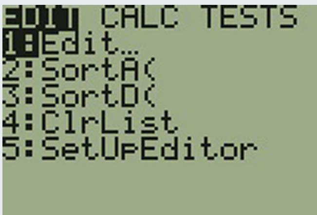
Figure 2.7.5 — The STAT menu. Choosing 1:Edit opens the list editor.
Step 3 — Enter midpoints and frequencies. Put the midpoints into L1 and the frequencies into L2.
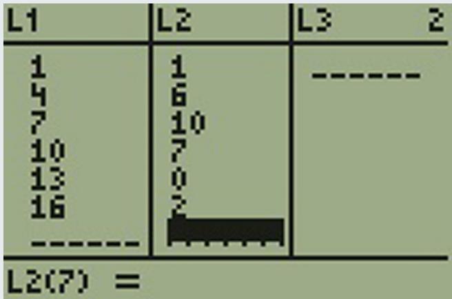
Figure 2.7.6 — The six midpoints in L1 beside their six frequencies in L2.
Step 4 — Run 1-Var Stats on the pair of lists. Press STAT, arrow across to CALC, and choose 1:1-Var Stats.
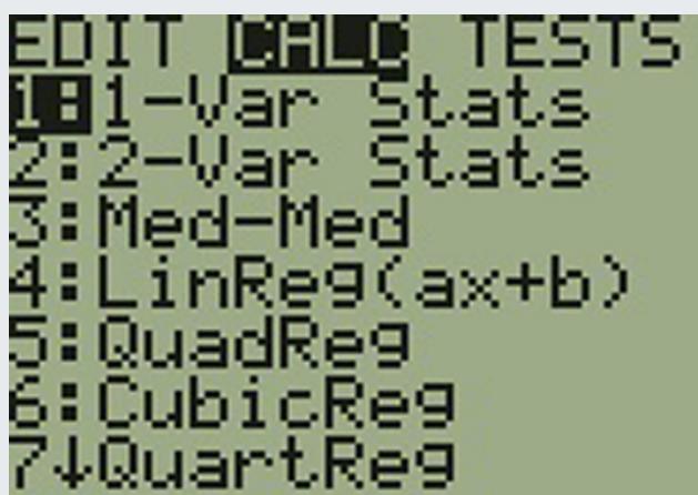
Figure 2.7.7 — The CALC tab of the STAT menu, with 1-Var Stats as the first entry.
Step 5 — Name both lists. Enter 2nd 1 for L1, a comma, then 2nd 2 for L2, and press ENTER.
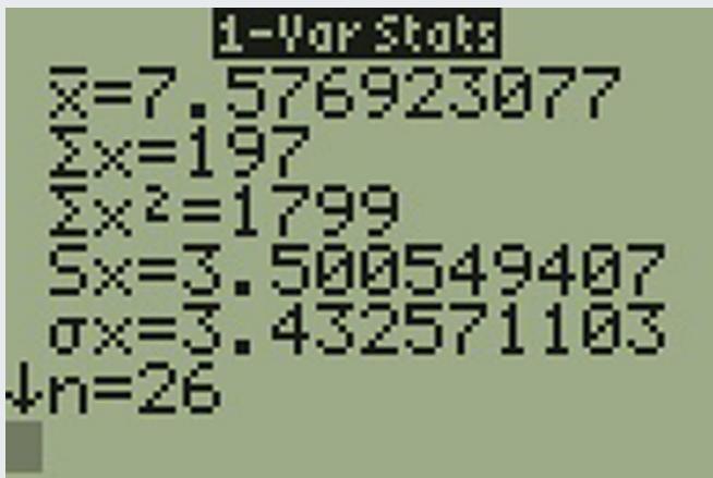
Figure 2.7.8 — The 1-Var Stats output. Both a population standard deviation and a sample standard deviation are displayed.
Answer: The screen displays both \(\sigma_x = 3.4326\) and \(s_x = 3.5005\). The data are a sample, so the answer is \(s_x \approx 3.50\) — the same value the table method produced, and \(\bar{x} = 7.5769\) matches the estimated mean of 7.58. Reading \(\sigma_x\) here would be the mistake to avoid.
Find the standard deviation for the data in Table 2.7.4.
| Class | \(f\) | \(m\) | \(f m\) | \(m - \bar{x}\) | \((m - \bar{x})^2\) | \(f(m - \bar{x})^2\) |
|---|---|---|---|---|---|---|
| 0-2 | 1 | 1 | 1 | -6.58 | 43.2964 | 43.2964 |
| 3-5 | 6 | 4 | 24 | -3.58 | 12.8164 | 76.8984 |
| 6-8 | 10 | 7 | 70 | -0.58 | 0.3364 | 3.3640 |
| 9-11 | 7 | 10 | 70 | 2.42 | 5.8564 | 40.9948 |
| 12-14 | 0 | 13 | 0 | 5.42 | 29.3764 | 0 |
| 15-17 | 2 | 16 | 32 | 8.42 | 70.8964 | 141.7928 |
| SUM | 26 | 197 | 306.3464 |
Solution
Step 1 — The estimated mean. The second, third, and fourth columns give it: multiply each midpoint by its frequency, total the products, and divide by the total frequency.
$$\bar{x} = \frac{\Sigma f m}{\Sigma f} = \frac{197}{26} \approx 7.58$$Step 2 — Fill the deviation columns. With \(\bar{x}\) in hand, subtract it from each midpoint to get \(m - \bar{x}\), square each difference, then multiply by that class's frequency. The final column totals 306.3464.
Step 3 — Apply the sample formula. The data are treated as a sample, so divide by \(n - 1 = 25\):
$$s_x = \sqrt{\frac{\Sigma f(m - \bar{x})^2}{n - 1}} = \sqrt{\frac{306.3464}{26 - 1}} = \sqrt{12.2539} \approx 3.50$$Answer: \(s_x \approx 3.50\). The formula is not complicated, but these calculations are normally performed with technology — notice that the 12-14 class contributes nothing to the total because its frequency is zero, even though its midpoint sits well away from the mean.
Try it in rāSHio
The calculator above takes a frequency list, but rāSHio's panels each read a single column, so there is nowhere to put your frequencies: Stats → Summary Statistics will not weight the midpoints, and Graph → Frequency Table counts raw observations rather than accepting counts you already have. Enter the table the way it is actually defined instead. Paste the 26 values with File → Delimited List, each midpoint repeated as many times as its frequency — 1 once, 4 six times, 7 ten times, 10 seven times, 16 twice, and 13 not at all — and Stats → Summary Statistics returns \(\bar{x} = 7.5769\) and \(s_x = 3.5005\), this example's answers exactly, with \(\sigma_x = 3.4326\) beside them as the trap to avoid. Typing the list out is not a workaround; it is the grouped-data assumption made literal, every value in a class treated as though it sat on the midpoint. What that frees you to spend attention on is the part that actually needs judgement: whether the midpoints are a fair stand-in for the values you cannot see.
Figure 2.7.9 — Where a grouped table comes from: Graph → Frequency Table counts raw values into one row each. It runs the opposite direction from this example, which starts from a table that already exists — use it when you have the observations and want the table, and the note above when you have the table and want \(s_x\).
2.7.4 Comparing Values from Different Data Sets
The number of standard deviations a value lies from its mean is called its z-score, written \(z\). A positive \(z\) means the value is above its mean, a negative \(z\) means it is below, and \(z = 0\) means the value equals the mean.
Summary of the z-score formulas. The table below collects the sample and population forms for quick reference.
| Data set | Value from a z-score | z-score from a value |
|---|---|---|
| Sample | \(x = \bar{x} + z s\) | \(z = \dfrac{x - \bar{x}}{s}\) |
| Population | \(x = \mu + z \sigma\) | \(z = \dfrac{x - \mu}{\sigma}\) |
One caution before the example: pay careful attention to signs, and to which direction counts as better in the context. For a GPA, higher is better, so a higher z-score wins. For a race time, lower is better, so the more negative z-score wins. The arithmetic does not know which you meant.
The standard deviation earns its keep when you compare values that come from different data sets. If the two sets have different means and different standard deviations, comparing the raw values directly can be misleading — a 77 out of 100 and a 2.85 out of 4 are not on the same scale, and neither are a 26-second swim and a 27-second swim from two teams of different quality.
The fix is to stop comparing the values and compare their positions instead. For each data value, calculate how many standard deviations away from its own mean the value is. That is the same equation as before, solved for the count:
$$\#\text{ofSTDEVs} = \frac{\text{value} - \text{mean}}{\text{standard deviation}}$$Now the two numbers are directly comparable, because both are measured in standard deviations of their own data set rather than in points or seconds.
Definition 2.7.6 — Two GPAs on incompatible scales drop onto one shared z-axis, where they can finally be compared.
Two swimmers, Drew Halloran and Tomás Vega, from different teams, wanted to find out who had the faster time for the 50 meter freestyle compared to his own team. Which swimmer had the faster time when compared to his team?
| Swimmer | Time (seconds) | Team Mean Time | Team Standard Deviation |
|---|---|---|---|
| Drew | 26.2 | 27.2 | 0.8 |
| Tomás | 27.3 | 30.1 | 1.4 |
Solution
Step 1 — Drew's z-score.
$$z = \frac{26.2 - 27.2}{0.8} = \frac{-1.0}{0.8} = -1.25$$Step 2 — Tomás's z-score.
$$z = \frac{27.3 - 30.1}{1.4} = \frac{-2.8}{1.4} = -2.0$$Step 3 — Decide which direction is better. These are race times, so a lower time is better and a negative z-score is good. Tomás swam 2 standard deviations faster than his team's mean; Drew swam 1.25 standard deviations faster than his.
Answer: Tomás had the faster time compared to his team. Note that Drew's raw time of 26.2 seconds is the quicker of the two, so comparing raw times would have given the opposite answer — Tomás's team is simply slower overall, and the z-score is what corrects for that.
Two students, Mei Lin Chen and Hannah Brenner, from different high schools, wanted to find out who had the higher GPA compared to her own school. Which student had the higher GPA when compared to her school?
| Student | GPA | School Mean GPA | School Standard Deviation |
|---|---|---|---|
| Mei Lin | 2.85 | 3.0 | 0.7 |
| Hannah | 77 | 80 | 10 |
Solution
Step 1 — Set up the right comparison. The two GPAs are on different scales, so compare z-scores instead of raw values:
$$z = \#\text{ofSTDEVs} = \frac{\text{value} - \text{mean}}{\text{standard deviation}} = \frac{x - \mu}{\sigma}$$Step 2 — Mei Lin's z-score.
$$z = \frac{2.85 - 3.0}{0.7} = \frac{-0.15}{0.7} \approx -0.21$$Step 3 — Hannah's z-score.
$$z = \frac{77 - 80}{10} = \frac{-3}{10} = -0.3$$Step 4 — Compare, watching the signs. Both students are below their school's mean. Mei Lin is 0.21 standard deviations below; Hannah is 0.3 standard deviations below. For a GPA, higher values are better, and \(-0.21\) is higher than \(-0.3\).
Answer: Mei Lin has the better GPA compared to her school. Neither student is above average at her own school, but Mei Lin is closer to her school's mean than Hannah is to hers.
2.7.5 How Much of the Data Falls Close to the Mean
The two-standard-deviation rule of thumb from the start of this section can be made sharper. A few facts give more insight into what the standard deviation tells us about the distribution of the data, and they come in two versions: one that holds no matter what the data look like, and a stronger one that holds only for bell-shaped data.
For ANY data set, no matter what the distribution of the data is:
- At least 75% of the data is within two standard deviations of the mean.
- At least 89% of the data is within three standard deviations of the mean.
- At least 95% of the data is within 4.5 standard deviations of the mean.
For data having a distribution that is BELL-SHAPED and SYMMETRIC:
- Approximately 68% of the data is within one standard deviation of the mean.
- Approximately 95% of the data is within two standard deviations of the mean.
- More than 99% of the data is within three standard deviations of the mean.
The Empirical Rule applies only when the shape of the distribution is bell-shaped and symmetric — which is exactly why Section 2.6 spent its time teaching you to name a shape. Use the wrong rule and your conclusion is wrong. We will learn more about this when we study the normal, or Gaussian, probability distribution in later chapters.
Two quick screens are in common use. One flags a value sitting more than \(1.5 \times \text{IQR}\) beneath \(Q_1\) or above \(Q_3\); the other flags a value more than two standard deviations from the mean. Neither is a test — each is a prompt to go look harder at a suspicious value.
No real variable is exactly normal, yet a great many come close enough that the bell curve describes them well. That closeness is why we reach for it so often — to stand in for raw data and, later on, for probability distributions.
Sketch the curve before you compute anything. Mark the mean, shade the region the question is asking about, and read a rough probability straight off your own drawing. Convert the value you care about into a z-score second — that order leaves you with an estimate to check the exact answer against.
Two more habits belong here, both about getting the data into the machine correctly before you trust anything it reports.
Reach the STAT screen from the main MENU by pressing 2. The left and right arrows move you between lists, so highlight whichever one you want to fill. Type a value, press EXE to lock it in, and the cursor drops to the next row ready for the following one.
With your values already loaded into L1, press 2ND Y= to reach STAT PLOT and switch the first plot to ON. The plot-type row holds several icons; move right to the fourth, which draws a box plot with outliers marked as separate dots. Set Xlist to L1 and leave Freq at 1. Finish with ZOOM and 9:ZoomStat, which sizes the window around your data for you.
When you describe any distribution, comment on all three of its important characteristics — center, spread, and shape — and note any especially unusual cases. Sections 2.5, 2.6, and 2.7 gave you one each. A description that reports only the average is not a description of the data.
A standardized test has a bell-shaped, symmetric score distribution with a mean of 500 and a standard deviation of 100.
a. Approximately what percentage of test-takers score between 300 and 700?
b. A different test has a mean of 500 and a standard deviation of 100 but a strongly skewed distribution. What is the most you can say about the percentage scoring between 300 and 700?
Solution
Step 1 — Translate the interval into standard deviations (part a). The scores 300 and 700 sit at
$$z = \frac{300 - 500}{100} = -2 \qquad z = \frac{700 - 500}{100} = 2$$so the interval is exactly two standard deviations either side of the mean.
Step 2 — Pick the right rule. The distribution is bell-shaped and symmetric, so the Empirical Rule applies: approximately 95% of the data is within two standard deviations of the mean.
Step 3 — Handle the skewed case (part b). The Empirical Rule is off the table because the shape requirement fails. Chebyshev's Rule holds for any distribution, and it says at least 75% of the data is within two standard deviations of the mean.
Answer: For the bell-shaped test, about 95% of test-takers score between 300 and 700. For the skewed test, you can only say that at least 75% do — the true figure could be anywhere from 75% up, and without knowing the shape you cannot pin it down further.
Problem Set 2.7
The following data are the distances between 20 retail stores and a large distribution center, in miles. Use them for problems 1 and 2.
29; 37; 38; 40; 58; 67; 68; 69; 76; 86; 87; 95; 96; 96; 99; 106; 112; 127; 145; 150
Problem 1. Use a graphing calculator or computer to find the standard deviation and round to the nearest tenth.
Solution
Step 1 — Find the mean first. The 20 distances total 1,681 miles, so
$$\bar{x} = \frac{1{,}681}{20} = 84.05 \text{ miles.}$$Step 2 — Enter the data and read the standard deviation. These 20 stores are a sample, so read \(Sx\) rather than \(\sigma x\) from 1-VarStats:
Note on the graphing calculator. Put all 20 distances in L1, leave the frequency argument blank, and run STAT CALC 1:1-VarStats. The screen reports \(\bar{x} = 84.05\), \(Sx = 34.5169\ldots\), and \(\sigma x = 33.6429\ldots\), with \(n = 20\).
Answer: \(s \approx 34.5\) miles. (Had the 20 stores been the entire population, the answer would be \(\sigma \approx 33.6\) miles.)
Problem 2. Find the value that is one standard deviation below the mean.
Solution
Step 1 — Recall the equation. A value one standard deviation below the mean is \(\text{value} = \bar{x} + (-1)(s)\).
Step 2 — Substitute the mean and standard deviation from the previous problem.
$$\text{value} = 84.05 + (-1)(34.5169) = 49.53$$Answer: About 49.5 miles. A store 49.5 miles from the distribution center is one standard deviation closer than average.
Problem 3. Two baseball players, Fredo and Karl, on different teams wanted to find out who had the higher batting average when compared to his team. Which baseball player had the higher batting average when compared to his team?
| Baseball Player | Batting Average | Team Batting Average | Team Standard Deviation |
|---|---|---|---|
| Fredo | 0.158 | 0.166 | 0.012 |
| Karl | 0.177 | 0.189 | 0.015 |
Solution
Step 1 — Recognize that the two averages are not comparable directly. The two players bat in different leagues with different team means and different team spreads, so compare z-scores instead of raw averages.
Step 2 — Fredo's z-score.
$$z = \frac{0.158 - 0.166}{0.012} = \frac{-0.008}{0.012} \approx -0.67$$Step 3 — Karl's z-score.
$$z = \frac{0.177 - 0.189}{0.015} = \frac{-0.012}{0.015} = -0.80$$Step 4 — Decide which direction is better. For a batting average, higher is better, so the larger z-score wins. Both players are below their own team's average, but \(-0.67\) is larger than \(-0.80\).
Answer: Fredo had the higher batting average when compared to his team. His raw average of 0.158 is the lower of the two, so comparing raw averages would give the wrong answer — Karl simply plays on a team that hits better overall.
Problem 4. Use Table 2.7.7 to find, for each player's team, the batting average that is three standard deviations
a) above the team mean;
b) below the team mean.
Solution
Step 1 — Set up the equation for each team. Three standard deviations from a team mean is \(\text{value} = \text{mean} + (\pm 3)(s)\), applied with that team's own mean and standard deviation.
Step 2 — Fredo's team (mean 0.166, standard deviation 0.012), part a and part b.
$$0.166 + (3)(0.012) = 0.202 \qquad 0.166 - (3)(0.012) = 0.130$$Step 3 — Karl's team (mean 0.189, standard deviation 0.015), part a and part b.
$$0.189 + (3)(0.015) = 0.234 \qquad 0.189 - (3)(0.015) = 0.144$$Answer: a) Three standard deviations above the mean is 0.202 for Fredo's team and 0.234 for Karl's team. b) Three standard deviations below the mean is 0.130 for Fredo's team and 0.144 for Karl's team. By Chebyshev's Rule at least 89% of each team's batting averages fall inside its own interval.
Problem 5. Find the standard deviation for each of the following frequency tables using the formula, then check your calculations with a TI-83/84.
a)
| Grade | Frequency |
|---|---|
| 49.5-59.5 | 2 |
| 59.5-69.5 | 3 |
| 69.5-79.5 | 8 |
| 79.5-89.5 | 12 |
| 89.5-99.5 | 5 |
b)
| Daily Low Temperature | Frequency |
|---|---|
| 49.5-59.5 | 53 |
| 59.5-69.5 | 32 |
| 69.5-79.5 | 15 |
| 79.5-89.5 | 1 |
| 89.5-99.5 | 0 |
c)
| Points per Game | Frequency |
|---|---|
| 49.5-59.5 | 14 |
| 59.5-69.5 | 32 |
| 69.5-79.5 | 15 |
| 79.5-89.5 | 23 |
| 89.5-99.5 | 2 |
Solution
Step 1 — Find each class midpoint. Average the two endpoints of every class. For all three tables the midpoints are 54.5, 64.5, 74.5, 84.5, and 94.5.
Step 2 — Table 2.7.8, the grades (part a). With frequencies 2, 3, 8, 12, 5 the total is \(n = 30\) and
$$\bar{x} = \frac{\Sigma f m}{\Sigma f} = \frac{2{,}385}{30} = 79.5$$The squared-deviation column totals \(\Sigma f(m - \bar{x})^2 = 3{,}550\), so
$$s = \sqrt{\frac{3{,}550}{30 - 1}} = \sqrt{122.41} \approx 11.1$$Step 3 — Table 2.7.9, the daily low temperatures (part b). With frequencies 53, 32, 15, 1, 0 the total is \(n = 101\) and
$$\bar{x} = \frac{6{,}154.5}{101} \approx 60.94$$Here \(\Sigma f(m - \bar{x})^2 \approx 5{,}916.9\), so
$$s = \sqrt{\frac{5{,}916.9}{101 - 1}} = \sqrt{59.17} \approx 7.7$$Step 4 — Table 2.7.10, the points per game (part c). With frequencies 14, 32, 15, 23, 2 the total is \(n = 86\) and
$$\bar{x} = \frac{6{,}077}{86} \approx 70.66$$Here \(\Sigma f(m - \bar{x})^2 \approx 10{,}633.8\), so
$$s = \sqrt{\frac{10{,}633.8}{86 - 1}} = \sqrt{125.10} \approx 11.2$$Note on the graphing calculator. For each table, put the five midpoints in L1 and that table's frequencies in L2, then run 1-VarStats L1, L2. The \(Sx\) value on the screen matches the hand calculation in each case.
Answer: a) \(s \approx 11.1\); b) \(s \approx 7.7\); c) \(s \approx 11.2\). The temperature data are the most tightly clustered of the three, even though they have by far the largest \(n\) — a bigger sample does not mean a bigger spread.
The population parameters below describe the full-time equivalent number of students (FTES) each year at a local community college over a 29-year period. Use them for problems 6 through 11.
- \(\mu = 1{,}000\) FTES
- median \(= 1{,}014\) FTES
- \(\sigma = 474\) FTES
- first quartile \(= 528.5\) FTES
- third quartile \(= 1{,}447.5\) FTES
- \(n = 29\) years
Problem 6. A sample of 11 years is taken. About how many are expected to have a FTES of 1,014 or above? Explain how you determined your answer.
Solution
Step 1 — Notice which statistic 1,014 is. The problem gives the median as 1,014 FTES.
Step 2 — Use what the median means. The median splits the data in half: 50% of the 29 years are at or below 1,014 FTES and 50% are at or above it.
Step 3 — Apply that fraction to the sample of 11.
$$(0.50)(11) = 5.5$$Answer: About 6 years (5 or 6 in practice, since you cannot have half a year). Because 1,014 FTES is the median, half of all years sit at or above it, so half of any sample of 11 years is the expected count.
Problem 7. 75% of all years have an FTES:
a) at or below what value?
b) at or above what value?
Solution
Step 1 — Translate 75% at or below into a quartile. The value with 75% of the data at or below it is the third quartile, \(Q_3\).
Step 2 — Translate 75% at or above into a quartile. The value with 75% of the data at or above it has 25% at or below it, which is the first quartile, \(Q_1\).
Step 3 — Read both from the given parameters. \(Q_3 = 1{,}447.5\) FTES and \(Q_1 = 528.5\) FTES.
Answer: a) At or below 1,447.5 FTES. b) At or above 528.5 FTES.
Problem 8. What is the population standard deviation?
Solution
Step 1 — Find the symbol for a population standard deviation. A population standard deviation is written \(\sigma\), not \(s\), and the problem states these parameters describe the full 29-year population.
Step 2 — Read it off the given list.
Answer: \(\sigma = 474\) FTES. Because these are population parameters, the correct symbol is \(\sigma\); using \(s\) would claim the 29 years were only a sample.
Problem 9. What percent of the FTES were from 528.5 to 1,447.5? How do you know?
Solution
Step 1 — Identify the two endpoints. 528.5 FTES is \(Q_1\) and 1,447.5 FTES is \(Q_3\).
Step 2 — Use what the quartiles mean. \(Q_1\) has 25% of the data at or below it and \(Q_3\) has 75% at or below it, so the stretch between them holds \(75\% - 25\% = 50\%\) of the data.
Answer: 50% of the years had an FTES between 528.5 and 1,447.5. We know it because those two numbers are the first and third quartiles, and by definition the quartiles cut off the middle half of the data.
Problem 10. What is the IQR? What does the IQR represent?
Solution
Step 1 — Recall the definition. The interquartile range is \(\text{IQR} = Q_3 - Q_1\).
Step 2 — Substitute.
$$\text{IQR} = 1{,}447.5 - 528.5 = 919$$Answer: \(\text{IQR} = 919\) FTES. It represents the spread of the middle 50% of the years — the width of the range that the typical half of the data occupies, with the smallest quarter and the largest quarter of the years both excluded.
Problem 11. How many standard deviations away from the mean is the median?
Solution
Step 1 — Set up the z-score. The question asks for \(\#\text{ofSTDEVs}\), which is the z-score of the median treated as a value in the population.
$$z = \frac{x - \mu}{\sigma}$$Step 2 — Substitute the median for \(x\).
$$z = \frac{1{,}014 - 1{,}000}{474} = \frac{14}{474} \approx 0.03$$Answer: About 0.03 standard deviations above the mean — essentially zero. The mean and the median are so close together that, on the scale of this data's spread, they are the same number. From Section 2.6, that is what a roughly symmetrical distribution looks like.
The population FTES for a specific six-year period was given in an updated report. Use Table 2.7.11 for problems 12 through 14.
| Year | 1 | 2 | 3 | 4 | 5 | 6 |
|---|---|---|---|---|---|---|
| Total FTES | 1,585 | 1,690 | 1,735 | 1,935 | 2,021 | 1,890 |
Problem 12. Calculate the mean, median, standard deviation, the first quartile, the third quartile, and the IQR. Round to one decimal place.
Solution
Step 1 — The mean. The six values total 10,856 FTES, so
$$\bar{x} = \frac{10{,}856}{6} \approx 1{,}809.3 \text{ FTES.}$$Step 2 — The median. Ordered, the values are 1,585; 1,690; 1,735; 1,890; 1,935; 2,021. With six values the median is the average of the 3rd and 4th:
$$M = \frac{1{,}735 + 1{,}890}{2} = 1{,}812.5 \text{ FTES.}$$Step 3 — The standard deviation. The squared deviations from 1,809.3 total about 137,193. These six years are described as the population, so divide by \(N = 6\):
$$\sigma = \sqrt{\frac{137{,}193}{6}} = \sqrt{22{,}865.6} \approx 151.2 \text{ FTES.}$$Step 4 — The quartiles. Split the ordered list at the median. The lower half is 1,585; 1,690; 1,735, whose median is \(Q_1 = 1{,}690\). The upper half is 1,890; 1,935; 2,021, whose median is \(Q_3 = 1{,}935\).
Step 5 — The IQR.
$$\text{IQR} = 1{,}935 - 1{,}690 = 245 \text{ FTES.}$$Answer: \(\bar{x} \approx 1{,}809.3\); median \(= 1{,}812.5\); \(\sigma \approx 151.2\); \(Q_1 = 1{,}690\); \(Q_3 = 1{,}935\); \(\text{IQR} = 245\), all in FTES. (Treating the six years as a sample instead would give \(s \approx 165.6\). The interpolation formula from Section 2.3 gives slightly different quartiles, \(Q_1 \approx 1{,}663.8\) and \(Q_3 \approx 1{,}956.5\); a TI-84 reports the median-of-halves values above.)
Problem 13. What additional information is needed to construct a box plot for the FTES for Years 1 to 6 and a box plot for the 29-year period shown earlier?
Solution
Step 1 — List what a box plot needs. A box plot is drawn from the five-number summary: the smallest value, \(Q_1\), the median, \(Q_3\), and the largest value.
Step 2 — Check the six-year data against that list. We have the full list of six values, so the smallest (1,585) and largest (2,021) are already known along with the three middle numbers. Nothing further is needed.
Step 3 — Check the 29-year data. For that period we were given only \(\mu\), the median, \(\sigma\), \(Q_1\), and \(Q_3\). The two ends of the whiskers are missing.
Answer: For the 29-year period you need the smallest and the largest FTES values — the minimum and maximum that complete the five-number summary. For Years 1 to 6 no additional information is needed, because the raw data list supplies the minimum and maximum directly.
Problem 14. Compare the standard deviation for the previous 29-year period with the standard deviation for the six-year period shown in Table 2.7.11. Why do you suppose the standard deviations are so different?
Solution
Step 1 — Put the two figures side by side. The 29-year period has \(\sigma = 474\) FTES. The six-year period has \(\sigma \approx 151.2\) FTES.
Step 2 — Compare them. The 29-year standard deviation is more than three times the six-year one.
Step 3 — Explain why the window matters. Over 29 years the college grew, so the FTES values run from small early-year enrollments up to much larger recent ones, and the standard deviation has to cover that whole climb. Six consecutive years catch only a short stretch of the same trend, where every value sits within a few hundred FTES of the others.
Answer: The 29-year standard deviation is about three times larger. A longer time window captures more of the college's growth, so the values it contains are spread over a much wider range. The six-year window is short enough that enrollment barely changed across it, which is why its spread is small.
Problem 15. Three students were applying to the same graduate school. They came from schools with different grading systems. Which student had the best GPA when compared to other students at his or her school? Explain how you determined your answer.
| Student | GPA | School Average GPA | School Standard Deviation |
|---|---|---|---|
| Thuy | 2.7 | 3.2 | 0.8 |
| Vichet | 87 | 75 | 20 |
| Kamala | 8.6 | 8 | 0.4 |
Solution
Step 1 — Recognize the three grading systems are different scales. A 2.7, an 87, and an 8.6 cannot be compared directly, so compute each student's z-score against their own school.
Step 2 — Thuy's z-score.
$$z = \frac{2.7 - 3.2}{0.8} = \frac{-0.5}{0.8} = -0.625$$Step 3 — Vichet's z-score.
$$z = \frac{87 - 75}{20} = \frac{12}{20} = 0.6$$Step 4 — Kamala's z-score.
$$z = \frac{8.6 - 8}{0.4} = \frac{0.6}{0.4} = 1.5$$Step 5 — Compare. For a GPA, higher is better, so the largest z-score wins: \(1.5 > 0.6 > -0.625\).
Answer: Kamala had the best GPA compared to other students at her school — she is 1.5 standard deviations above her school's average, while Vichet is 0.6 above his and Thuy is 0.625 below hers. Note that Vichet's raw 87 is the largest number on the list and he still does not win.
Problem 16. A music school has budgeted to purchase three musical instruments. They plan to purchase a piano costing $3,000, a guitar costing $550, and a drum set costing $600. The mean cost for a piano is $4,000 with a standard deviation of $2,500. The mean cost for a guitar is $500 with a standard deviation of $200. The mean cost for drums is $700 with a standard deviation of $100. Which cost is the lowest when compared to other instruments of the same type? Which cost is the highest when compared to other instruments of the same type? Justify your answer.
Solution
Step 1 — Set up a z-score for each instrument against its own market.
Step 2 — The piano.
$$z = \frac{3{,}000 - 4{,}000}{2{,}500} = \frac{-1{,}000}{2{,}500} = -0.4$$Step 3 — The guitar.
$$z = \frac{550 - 500}{200} = \frac{50}{200} = 0.25$$Step 4 — The drum set.
$$z = \frac{600 - 700}{100} = \frac{-100}{100} = -1.0$$Step 5 — Compare, remembering which direction is which. The most negative z-score is the cheapest relative to its own market; the largest is the most expensive.
Answer: The drum set is the lowest cost when compared to other drum sets, at 1.0 standard deviation below the mean drum price. The guitar is the highest, at 0.25 standard deviations above the mean guitar price. The piano is the most expensive item in raw dollars, at $3,000, yet it is a comparative bargain — 0.4 standard deviations below the mean piano price.
Problem 17. An elementary school class ran one mile with a mean of 11 minutes and a standard deviation of three minutes. Yasmin Haddad, a student in the class, ran one mile in eight minutes, her best time so far. A junior high school class ran one mile with a mean of nine minutes and a standard deviation of two minutes. Kenji, a student in the class, ran one mile in 8.5 minutes. A high school class ran one mile with a mean of seven minutes and a standard deviation of four minutes. Nedda, a student in the class, ran one mile in eight minutes.
a) Why is Kenji considered a better runner than Nedda, even though Nedda ran faster than he did?
b) Who is the fastest runner with respect to their class? Explain why.
Solution
Step 1 — Compute a z-score for each runner against their own class.
Step 2 — Yasmin's z-score.
$$z = \frac{8 - 11}{3} = -1.0$$Step 3 — Kenji's z-score.
$$z = \frac{8.5 - 9}{2} = -0.25$$Step 4 — Nedda's z-score.
$$z = \frac{8 - 7}{4} = 0.25$$Step 5 — Read the signs (part a). These are times, so a negative z-score means faster than the class average. Kenji's \(-0.25\) puts him below his class mean; Nedda's \(+0.25\) puts her above hers.
Step 6 — Find the most negative z-score (part b). Comparing \(-1.0\), \(-0.25\), and \(0.25\), the most negative is Yasmin's.
Answer: a) Kenji ran a quarter of a standard deviation faster than his class average, while Nedda ran a quarter of a standard deviation slower than hers. Nedda's raw time of 8 minutes beats Kenji's 8.5 minutes, but she was racing a much faster class, so relative to her own classmates she is the weaker runner. b) Yasmin is the fastest with respect to her class, at 1.0 standard deviation below her class mean.
Problem 18. A selection of countries has poverty rates that range from 11.4% to 74.6%. This data is summarized in Table 2.7.13. What is the best estimate of the average poverty percentage for these countries? What is the standard deviation for the listed poverty rates? The United States has an average poverty rate of 33.9%. Is this rate above average or below? How unusual is the United States' rate compared to the average rate? Explain.
| Percent of Population | Number of Countries |
|---|---|
| 11.4-20.45 | 29 |
| 20.45-29.45 | 13 |
| 29.45-38.45 | 4 |
| 38.45-47.45 | 0 |
| 47.45-56.45 | 2 |
| 56.45-65.45 | 1 |
| 65.45-74.45 | 0 |
| 74.45-83.45 | 1 |
Solution
Step 1 — Find the class midpoints. Averaging each class's endpoints gives 15.925, 24.95, 33.95, 42.95, 51.95, 60.95, 69.95, and 78.95 percent.
Step 2 — Estimate the mean. The frequencies are 29, 13, 4, 0, 2, 1, 0, 1, so \(n = 50\) and \(\Sigma f m = 1{,}165.775\):
$$\bar{x} = \frac{1{,}165.775}{50} \approx 23.3\%$$Step 3 — Estimate the standard deviation. The squared-deviation column totals \(\Sigma f(m - \bar{x})^2 \approx 8{,}222.5\), so
$$s = \sqrt{\frac{8{,}222.5}{50 - 1}} = \sqrt{167.81} \approx 13.0\%$$Step 4 — Place the United States on that scale.
$$z = \frac{33.9 - 23.3}{13.0} \approx 0.82$$Step 5 — Judge how unusual that is. The rule of thumb calls a value unusual once it is more than two standard deviations from the mean. This one is less than one.
Answer: The best estimate of the average poverty percentage is about 23.3%, with a standard deviation of about 13.0%. At 33.9% the United States is above average, but only about 0.82 standard deviations above — well inside the two-standard-deviation line, so it is not an unusual rate for this group of countries.
Problem 19. Table 2.7.14 gives the percent of children under five considered to be underweight. What is the best estimate for the mean percentage of underweight children? What is the standard deviation? Which interval or intervals could be considered unusual? Explain.
| Percent of Underweight Children | Number of Countries |
|---|---|
| 16-21.45 | 23 |
| 21.45-26.9 | 4 |
| 26.9-32.35 | 9 |
| 32.35-37.8 | 7 |
| 37.8-43.25 | 6 |
| 43.25-48.7 | 1 |
Solution
Step 1 — Find the class midpoints. Averaging each class's endpoints gives 18.725, 24.175, 29.625, 35.075, 40.525, and 45.975 percent.
Step 2 — Estimate the mean. The frequencies are 23, 4, 9, 7, 6, 1, so \(n = 50\) and \(\Sigma f m = 1{,}328.65\):
$$\bar{x} = \frac{1{,}328.65}{50} \approx 26.6\%$$Step 3 — Estimate the standard deviation. The squared-deviation column totals \(\Sigma f(m - \bar{x})^2 \approx 3{,}573.8\), so
$$s = \sqrt{\frac{3{,}573.8}{50 - 1}} = \sqrt{72.94} \approx 8.5\%$$Step 4 — Mark the unusual boundary. More than two standard deviations from the mean counts as unusual, which here means below \(26.573 - 2(8.54) \approx 9.5\%\) or above \(26.573 + 2(8.54) \approx 43.7\%\).
Step 5 — Check each interval against that boundary. Only the top class, 43.25-48.7, has a midpoint (45.975) beyond 43.7%. Its z-score is
$$z = \frac{45.975 - 26.573}{8.54} \approx 2.27$$Answer: The best estimate of the mean is about 26.6% with a standard deviation of about 8.5%. The 43.25-48.7 interval could be considered unusual: its midpoint sits about 2.3 standard deviations above the mean, past the two-standard-deviation rule of thumb, and only one country falls in it. No interval reaches the unusual boundary on the low side, because the data stop at 16%.
Key Terms
standard deviation — a number that measures how far the data values are from their mean, in the same units as the data; written \(s\) for a sample and \(\sigma\) for a population.
variation — the extent to which data values differ from one another; also called spread.
deviation — the difference between a data value and the mean, \(x - \bar{x}\) for a sample or \(x - \mu\) for a population.
variance — the average of the squared deviations, written \(s^2\) for a sample and \(\sigma^2\) for a population; the standard deviation is its square root.
sampling variability of a statistic — how much a statistic changes from one sample to another.
standard error of the mean — the standard deviation of the sampling distribution of the mean, \(\sigma / \sqrt{n}\).
z-score — the number of standard deviations a value lies from its mean, \(z = (x - \bar{x})/s\) for a sample or \(z = (x - \mu)/\sigma\) for a population.
variability — the term for describing data with reference to its spread.
Chebyshev's Rule — for any distribution, at least 75% of the data lies within two standard deviations of the mean, at least 89% within three, and at least 95% within 4.5.
Empirical Rule — for a bell-shaped, symmetric distribution, about 68% of the data lies within one standard deviation of the mean, about 95% within two, and more than 99% within three.