5.2 Using the Normal Distribution
SLO 3
Describe and apply probability concepts and distributions.
Here a normal curve stops being a picture and starts answering questions: shade the region a sentence describes, then read it off as a probability or run it backwards to the score, hour, or diameter sitting at a given percentile.
Learning Objectives
By the end of this section, you will be able to:
- read a shaded area under a normal curve as a probability, and convert between the area to the left of a value and the area to its right;
- use technology to find \(P(x < a)\), \(P(x > a)\), and \(P(a < x < b)\) for any normal distribution;
- find the value \(k\) that sits at a given percentile, and state what it means in the original units;
- translate phrases like "at least", "at most", "the bottom quartile", and "the middle 50%" into the areas a calculator needs.
The last section built the standard normal distribution and showed how a \(z\)-score locates any value on it. This section puts that machinery to work. Almost every question a normal distribution is asked comes down to one of two shapes: you are given a value and asked for a probability, or you are given a probability and asked for the value. Learn to tell those two apart on sight and the rest of the section is bookkeeping.
5.2.1 Areas to the Left and to the Right
Everything starts with a picture. For a continuous random variable, probability is area under the curve, so a probability statement and a shaded region are two ways of saying the same thing. The shaded area in the following graph is the area to the left of \(x\), and that area is exactly the probability \(P(X < x)\). Normal tables, computers, and calculators all exist to hand you that number.
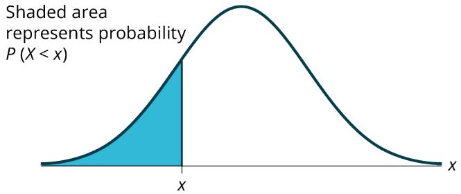
Figure 5.2.1 — The shaded area to the left of \(x\) represents the probability \(P(X < x)\).
The whole area under a normal curve is 1, so once you know one side you know the other. That gives the relationship you will use more than any other in this section:
$$ P(X > x) = 1 - P(X < x). $$Drawing the line through \(x\) slices the curve into exactly two pieces. Whichever piece the calculator hands you, subtracting from 1 gets you the other. You never have to compute a right tail directly.
Read it as a sentence rather than a formula. The quantity on the right is the area to the left of the vertical line drawn through the value, the quantity on the left is the area to the right of that same line, and together they fill the curve completely. Every problem in this section is some rearrangement of that one sentence, so it is worth saying out loud until it feels obvious. One more convenience comes free with continuous distributions: a strict inequality and a non-strict inequality describe the same probability. A single point has no width, so it has no area, and the difference between "less than" and "at most" vanishes entirely. That is not true for the discrete distributions of the last chapter, where a single value carries real probability and the difference between "fewer than five" and "at most five" is an entire outcome. Carrying that habit over from the discrete world is one of the most common sources of small, avoidable errors, so retire it deliberately rather than hoping it fades on its own. From here on, treat the four inequality symbols as two symbols with spare punctuation.
If the area to the left of \(x\) is 0.012, then what is the area to the right?
Solution
The two areas fill the whole curve, so they add to 1.
$$ \text{area to the right} = 1 - 0.012 = 0.988 $$Answer: The area to the right of \(x\) is 0.988.
If the area to the left is 0.0228, then what is the area to the right?
Solution
Step 1 — Name what you were given. The 0.0228 is the area to the left, which is \(P(X < x)\).
Step 2 — Subtract from the total area. The full area under any normal curve is 1.
$$ 1 - 0.0228 = 0.9772 $$Answer: The area to the right is 0.9772.
5.2.2 Calculations of Probabilities
For a normal random variable \(X\) and a number \(p\) with \(0 < p < 100\), the \(p^{\text{th}}\) percentile is the value \(k\) for which
$$ P(X < k) = \frac{p}{100}. $$Definition 5.2.1 - A percentile is a place on the axis: name the area and the boundary follows.
That is, \(p\) percent of the values are the same as or lower than \(k\), and the remaining \(100 - p\) percent are the same as or higher.
A value \(k\) located on the \(x\)-axis that separates a distribution into a specified area to its left and the remaining area to its right is called a critical value.
You can do all of this without technology using the probability tables in Appendix H. The tables carry their own instructions for how to read them, and they are what statisticians used for most of the twentieth century.
Both definitions describe the same point on the axis; "percentile" names it by the share of data below it, and "critical value" names it by the job it does of splitting the curve. You will meet critical values again in hypothesis testing, where the area to the right is chosen in advance and the value \(k\) is what you look up. For now the practical consequence is that any percentile question is an invNorm question, and any critical-value question is a percentile question wearing a different hat. The example below runs all four question types on one distribution: two probabilities and two percentiles, from the same set of exam scores.
Probabilities under a normal curve are calculated using technology. Instructions are given as necessary for the TI-83+ and TI-84 calculators, and the same two commands cover essentially every problem in this section. normalcdf takes a range of \(x\)-values and returns the area — that is the "value in, probability out" direction. invNorm takes an area and returns the \(x\)-value — that is the "probability in, value out" direction. Deciding which one a problem wants is the actual skill; typing it in is the easy part.
When a question hands you a percentage and asks for a score, a time, or a diameter, it is asking for a percentile, and the value it wants is traditionally called \(k\). The distinction matters enough to state carefully, because a large share of the errors students make in this section are not arithmetic errors at all — they are answering the wrong one of the two questions. If the problem ends with "what is the probability" or "what percent", the answer is a number between 0 and 1 and you want normalcdf. If the problem ends with a unit — points, hours, years, centimeters — the answer is a value on the \(x\)-axis and you want invNorm. Sketching the curve first makes this obvious: shade what the problem describes, then look at whether the thing you do not know is the shaded amount or the boundary of the shading.
The golf scores for a school team were normally distributed with a mean of 68 and a standard deviation of three. Find the probability that a randomly selected golfer scored less than 65.
Solution
Step 1 — Name the variable and its distribution. Let \(X\) = a golfer's score. Then \(X \sim N(68, 3)\), so \(\mu = 68\) and \(\sigma = 3\).
Step 2 — Decide which direction the question runs. It gives a score and asks for a probability, so this is normalcdf.
Step 3 — Compute. The lower bound is far out in the left tail.
$$ P(x < 65) = \text{normalcdf}(-10^{99}, 65, 68, 3) = 0.1587 $$Answer: The probability that a randomly selected golfer scored less than 65 is 0.1587, or about 16%.
The final exam scores in a statistics class were normally distributed with a mean of 63 and a standard deviation of five.
a. Find the probability that a randomly selected student scored more than 65 on the exam.
b. Find the probability that a randomly selected student scored less than 85.
c. Find the \(90^{\text{th}}\) percentile, that is, find the score \(k\) that has 90% of the scores below it and 10% of the scores above it.
d. Find the \(70^{\text{th}}\) percentile, that is, find the score \(k\) such that 70% of scores are below it and 30% of the scores are above it.
Solution
Part a — Set up. Let \(X\) = a score on the final exam. Then \(X \sim N(63, 5)\), where \(\mu = 63\) and \(\sigma = 5\). Draw a graph and shade the region to the right of 65, then find \(P(x > 65)\).
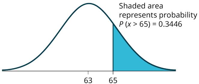
Figure 5.2.2 — The shaded right tail beyond a score of 65 on a \(N(63, 5)\) distribution. Its area is \(P(x > 65) = 0.3446\).
$$ P(x > 65) = 0.3446 $$On a TI-83/83+/84/84+: press 2nd DISTR, then 2:normalcdf(. The syntax is normalcdf(lower value, upper value, mean, standard deviation). For this problem, normalcdf(65,1E99,63,5) = 0.3446. You get 1E99 (which is \(10^{99}\)) by pressing 1, then the EE key (a 2nd key), then 99. The number \(10^{99}\) is so far out in the right tail that it stands in for infinity, so you are really calculating the area between 65 and the end of the curve. When the tail you want runs the other way, the lower bound becomes -1E99.
Before technology. The TI program calculates a \(z\)-score and then reads the probability off it. Before calculators, you did the same two moves by hand: compute the \(z\)-score, then look it up in a standard normal table that gave you the area to its left.
$$ z = \frac{65 - 63}{5} = 0.4 $$The table gives an area to the left of 0.6554, so
$$ P(x > 65) = P(z > 0.4) = 1 - 0.6554 = 0.3446, $$the same answer. The probability that any student selected at random scores more than 65 is 0.3446.
Part b — Set up. Draw a graph, shade everything to the left of 85, and find \(P(x < 85)\).
A score of 85 sits more than four standard deviations above the mean, so essentially the entire curve lies to its left.
$$ P(x < 85) = \text{normalcdf}(0, 85, 63, 5) = 1 \text{ (rounds to one)} $$The probability that one student scores less than 85 is approximately one, or 100%.
Part c — Set up. For each problem or part of a problem, draw a new graph. Draw the \(x\)-axis, then shade the area that corresponds to the \(90^{\text{th}}\) percentile.
Let \(k\) = the \(90^{\text{th}}\) percentile. The variable \(k\) is located on the \(x\)-axis, and \(P(x < k)\) is the area to the left of \(k\). The \(90^{\text{th}}\) percentile \(k\) separates the exam scores into those that are the same or lower than \(k\) and those that are the same or higher. Ninety percent of the test scores are the same as or lower than \(k\), and ten percent are the same as or higher. The variable \(k\) is often called a critical value.
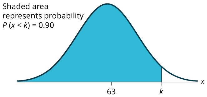
Figure 5.2.3 — The \(90^{\text{th}}\) percentile of the exam scores. The shaded region to the left of \(k\) holds 90% of the area.
$$ k = 69.4 $$On a TI-83/83+/84/84+: press 2nd DISTR, then 3:invNorm(. The syntax is invNorm(area to the left, mean, standard deviation). For this problem, invNorm(0.90,63,5) = 69.4.
The \(90^{\text{th}}\) percentile is 69.4. This means that 90% of the test scores fall at or below 69.4 and 10% fall at or above.
Part d — Set up. Draw a new graph and label it appropriately, shading the lower 70% of the area.
$$ k = \text{invNorm}(0.70, 63, 5) = 65.6 $$Answer: a. \(P(x > 65) = 0.3446\); b. \(P(x < 85) \approx 1\); c. the \(90^{\text{th}}\) percentile is 69.4; d. the \(70^{\text{th}}\) percentile is 65.6, so 70% of the test scores fall at or below 65.6 and 30% fall at or above.
Try it in rāSHio
Example 5.2.2 runs both directions on one distribution, and rāSHio runs them the same two ways. Choose Distributions → Normal, set mean 63 and standard deviation 5, then pick Right with cutoff 65 for part a’s 0.3446 and switch to Inverse (Left) with probability 0.90 for part c’s \(k = 69.4\) — the normalcdf and invNorm moves, one after the other on the same curve.
Figure 5.2.4 — Reading a tail area in rāSHio: Distributions → Normal, with the mean and standard deviation set by hand.
5.2.3 Probabilities Between Two Values
A "between" question shades a strip in the middle of the curve rather than a tail, and it is the easiest of the three shapes to compute: normalcdf already takes a lower bound and an upper bound, so you just supply both. The thinking happens before you type. Read the sentence and decide which number is the lower edge of the strip and which is the upper edge, because a swapped pair returns a negative area and there is no warning message.
A between-question asks how much of the population sits inside a window. "How many households use the computer between 1.8 and 2.75 hours" is the same question as "how tall is the pile of the density between those two marks".
The other question this subsection introduces is the quartile question, and it is a percentile question in disguise. The bottom quartile is the lowest 25% of the values, so its upper edge is the \(25^{\text{th}}\) percentile — an invNorm with an area of 0.25. Whenever a problem uses the words quarter, quartile, or median, translate it to a percentage first and then run the same machinery: bottom quartile is 0.25, median is 0.50, third quartile is 0.75. Nothing about the calculation changes, only the vocabulary the problem chose to hide the area behind, and that translation step is where almost all of the difficulty lives. Watch for the word "maximum" too, because it is the tell that a quartile question wants a value rather than a probability. Asking for the maximum time in the bottom quartile is asking for the boundary of that lowest quarter, which is a point on the axis, not an area under the curve. The example below runs one question of each direction on the same distribution, which is the pattern most exam questions follow: a probability first to get you comfortable with the numbers, then a percentile that reuses the same mean and standard deviation.
The golf scores for a school team were normally distributed with a mean of 68 and a standard deviation of three. Find the probability that a golfer scored between 66 and 70.
Solution
Step 1 — Set up. Let \(X\) = a golfer's score, so \(X \sim N(68, 3)\).
Step 2 — Identify the strip. The lower edge is 66 and the upper edge is 70.
Step 3 — Compute.
$$ P(66 < x < 70) = \text{normalcdf}(66, 70, 68, 3) = 0.4950 $$Answer: The probability that a golfer scored between 66 and 70 is 0.4950, so just under half the team's scores land in that four-point window.
A personal computer is used for office work at home, research, communication, personal finances, education, entertainment, social networking, and a myriad of other things. Suppose that the average number of hours a household personal computer is used for entertainment is two hours per day. Assume the times for entertainment are normally distributed and the standard deviation for the times is half an hour.
a. Find the probability that a household personal computer is used for entertainment between 1.8 and 2.75 hours per day.
b. Find the maximum number of hours per day that the bottom quartile of households uses a personal computer for entertainment.
Solution
Part a — Set up. Let \(X\) = the amount of time (in hours) a household personal computer is used for entertainment. Then \(X \sim N(2, 0.5)\), where \(\mu = 2\) and \(\sigma = 0.5\). We want \(P(1.8 < x < 2.75)\), which is the area between \(x = 1.8\) and \(x = 2.75\).
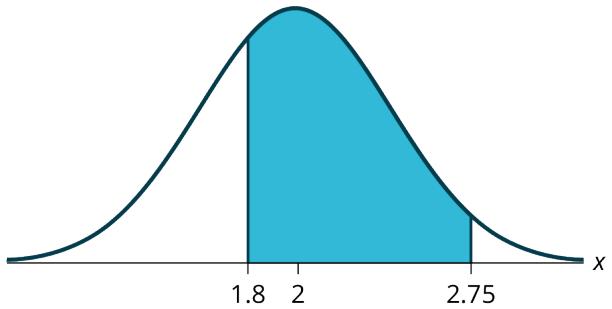
Figure 5.2.5 — The shaded strip between \(x = 1.8\) and \(x = 2.75\) hours under the \(N(2, 0.5)\) density.
$$ P(1.8 < x < 2.75) = \text{normalcdf}(1.8, 2.75, 2, 0.5) = 0.5886 $$The probability that a household personal computer is used between 1.8 and 2.75 hours per day for entertainment is 0.5886.
Part b — Translate the words. The bottom quartile is the lowest 25% of the times, so its maximum is the \(25^{\text{th}}\) percentile \(k\), the value with \(P(x < k) = 0.25\).
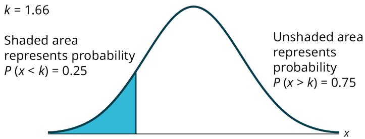
Figure 5.2.6 — The \(25^{\text{th}}\) percentile \(k = 1.66\). The shaded region holds 25% of the area and the unshaded region holds the other 75%.
$$ k = \text{invNorm}(0.25, 2, 0.5) = 1.66 $$Answer: a. \(P(1.8 < x < 2.75) = 0.5886\); b. the maximum number of hours per day that the bottom quartile of households uses a personal computer for entertainment is 1.66 hours.
Try it in rāSHio
The strip in part a is its own mode. In rāSHio choose Distributions → Normal, set mean 2 and standard deviation 0.5, pick Between with bounds 1.8 and 2.75 to get 0.5886, then switch to Inverse (Left) with probability 0.25 for part b’s bottom-quartile 1.66 hours.
5.2.4 Working with Percentiles
A percentile is only half an answer until you say what it means. Reporting "the \(80^{\text{th}}\) percentile is 48.6" tells a reader almost nothing on its own; "80% of smartphone users in this age range are 48.6 years old or younger" tells them everything. Getting into the habit of writing that sentence is worth real points on an exam and, more importantly, is the entire reason anyone computes a percentile in the first place.
Being at the \(80^{\text{th}}\) percentile does not mean you got 80% of something right. It means 80% of the group is at or below you. The percentile is your position in the line, not your grade.
The interpretation sentence has a fixed shape, and you can fill it in mechanically: [percent] of the [population] are [value] [units] or [less / more]. Notice what has to be true for the sentence to be honest. The percent comes from the area you fed into invNorm, the value comes back out of it, and the units are whatever the mean and standard deviation were stated in. If the problem gives ages in years, the percentile is a number of years — not a probability, not a percent, not a \(z\)-score. Students who lose points here almost always lost them by reporting a bare number with no units and no direction. The direction matters as much as the units, because the same value read the other way describes a completely different group: 48.6 years is the age that 80% of users are at or below, which also means only 20% of users are older than that. Both sentences are true and they describe the same computation, but a reader who is handed the wrong one walks away with the wrong picture of the population. Write the version the question asked for. If the problem says "find the percentile and interpret it", the interpretation belongs in the answer, not in your head. The example that follows works all three question shapes on one distribution and finishes with exactly that sentence.
In the United States the ages 13 to 55+ of smartphone users approximately follow a normal distribution with approximate mean and standard deviation of 36.9 years and 13.9 years, respectively.
a. Find the \(30^{\text{th}}\) percentile, and interpret it in a complete sentence.
b. What is the probability that the age of a randomly selected smartphone user in the range 13 to 55+ is less than 27 years old?
Solution
Part a — Percentile, so run invNorm.
The \(30^{\text{th}}\) percentile is 29.6 years. Thirty percent of smartphone users in the 13 to 55+ age range are 29.6 years old or younger.
Part b — Probability, so run normalcdf.
Answer: a. the \(30^{\text{th}}\) percentile is 29.6 years, meaning 30% of these smartphone users are 29.6 or younger; b. the probability that a randomly selected user is under 27 is 0.2382.
In the United States the ages 13 to 55+ of smartphone users approximately follow a normal distribution with approximate mean and standard deviation of 36.9 years and 13.9 years, respectively.
a. Determine the probability that a random smartphone user in the age range 13 to 55+ is between 23 and 64.7 years old.
b. Determine the probability that a randomly selected smartphone user in the age range 13 to 55+ is at most 50.8 years old.
c. Find the \(80^{\text{th}}\) percentile of this distribution, and interpret it in a complete sentence.
Solution
Part a — A between-question. Feed both edges to normalcdf.
Part b — "At most" is a left tail. For a continuous distribution, "at most 50.8" is the same as "less than 50.8", so the lower bound runs off to the left.
$$ \text{normalcdf}(-10^{99}, 50.8, 36.9, 13.9) = 0.8413 $$Part c — A percentile, so run invNorm.
The \(80^{\text{th}}\) percentile is 48.6 years. Eighty percent of the smartphone users in the age range 13 to 55+ are 48.6 years old or less.
Answer: a. 0.8186; b. 0.8413; c. 48.6 years, meaning 80% of these users are 48.6 or younger.
5.2.5 Quartiles, the IQR, and At Least Questions
Two more phrasings show up constantly, and both are handled by turning the words into an area before you touch the calculator.
The first is the interquartile range. You already know \(IQR = Q_3 - Q_1\) from the chapter on descriptive statistics; for a normal distribution you get \(Q_1\) and \(Q_3\) from invNorm at 0.25 and 0.75, then subtract. Nothing new happens, but the intermediate values are worth carrying to four decimal places, because subtracting two rounded numbers can shift the last digit of the answer.
\(Q_1\) and \(Q_3\) are places on the axis; the distance between them is a spread. Two distributions can share an IQR while sitting nowhere near each other.
The second phrasing is "at least", and it is the one that trips people up. "At least \(k\)" translates to \(x \geq k\), which is the area to the right of \(k\). But invNorm only accepts an area to the left. So a problem that says "forty percent of users are at least what age" is handing you a right-hand area of 0.40, and the number you actually type is \(1 - 0.40 = 0.60\). Skipping that subtraction is the single most common error in this subsection, and it fails quietly: you still get a plausible-looking age back, just the wrong one, with nothing on the screen to warn you. The defense is to sketch first. Shade the region the sentence describes, look at where the shading sits relative to the unknown value, and if the shading is on the right, subtract before you type. A second check costs nothing: an area to the left below 0.5 has to return a value below the mean, and an area above 0.5 has to return a value above it. If you asked for an area of 0.60 on a distribution centered at 36.9 and the calculator hands back 33, you typed the wrong area, and you caught it in two seconds instead of two pages. The same phrase family includes "at most", "no more than", and "no fewer than", so build the habit on this one and the rest come free.
Two thousand students took an exam. The scores on the exam have an approximate normal distribution with a mean \(\mu = 81\) points and standard deviation \(\sigma = 15\) points.
a. Calculate the first- and third-quartile scores for this exam.
b. The middle 50% of the exam scores are between what two values?
Solution
Part a — Quartiles are percentiles. \(Q_1\) is the \(25^{\text{th}}\) percentile and \(Q_3\) is the \(75^{\text{th}}\).
$$ Q_1 = \text{invNorm}(0.25, 81, 15) = 70.9 $$ $$ Q_3 = \text{invNorm}(0.75, 81, 15) = 91.1 $$Part b — The middle 50% is exactly the span between the quartiles. By definition, 25% of the scores fall below \(Q_1\) and 25% fall above \(Q_3\), leaving half the scores in between.
Answer: a. \(Q_1 = 70.9\) points and \(Q_3 = 91.1\) points; b. the middle 50% of the exam scores are between 70.9 and 91.1 points.
In the United States the ages 13 to 55+ of smartphone users approximately follow a normal distribution with approximate mean and standard deviation of 36.9 years and 13.9 years respectively. Using this information, answer the following questions and round answers to one decimal place.
a. Calculate the interquartile range (IQR).
b. Forty percent of the smartphone users from 13 to 55+ are at least what age?
Solution
Part a — Get both quartiles, then subtract.
$$ IQR = Q_3 - Q_1 $$Calculate \(Q_3\), the \(75^{\text{th}}\) percentile, and \(Q_1\), the \(25^{\text{th}}\) percentile.
$$ \text{invNorm}(0.75, 36.9, 13.9) = Q_3 = 46.2754 $$ $$ \text{invNorm}(0.25, 36.9, 13.9) = Q_1 = 27.5246 $$ $$ IQR = Q_3 - Q_1 = 18.8 $$Part b — Convert the right-hand area to a left-hand area. Find \(k\) where \(P(x \geq k) = 0.40\), since "at least" translates to "greater than or equal to". That 0.40 is the area to the right, so the area to the left is
$$ 1 - 0.40 = 0.60. $$Now invNorm can be used, because it takes the area to the left.
Answer: a. \(IQR = 18.8\) years; b. forty percent of the smartphone users from 13 to 55+ are at least 40.4 years old.
Try it in rāSHio
This is the example where the subtraction bites, so watch it happen. In rāSHio choose Distributions → Normal, set mean 36.9 and standard deviation 13.9, and run Inverse (Left) three times: 0.25 and 0.75 give the quartiles whose difference is the IQR of 18.8, and 0.60 — not 0.40 — gives part b’s 40.4 years. Ask it for 0.40 too: the 33.4 it hands back is the below-the-mean answer this subsection warns you to catch.
5.2.6 The Middle of the Distribution
The last phrasing to decode is "the middle \(P\)%", as in "the middle 20% of mandarin oranges have diameters between what two values". This one needs a short piece of reasoning before any calculation happens.
If the middle \(P\)% sits in the center of the curve, then \(100 - P\) percent is left over for the two tails. The normal distribution is symmetric, so those tails are equal, and each one carries half of what is left. Once you have the tail area, the two boundaries are just percentiles: the lower boundary \(k_1\) is the percentile at the left tail area, and the upper boundary \(k_2\) is the percentile at the left tail area plus the middle chunk.
Work it through with the middle 20%. Subtracting gives \(1 - 0.20 = 0.80\) of the area outside the middle, so each tail has an area of 0.40. The lower boundary \(k_1\) is therefore the \(40^{\text{th}}\) percentile, and the upper boundary \(k_2\) is the \(60^{\text{th}}\) percentile, since \(0.40 + 0.20 = 0.60\). Two invNorm calls finish the job. Do this on paper the first few times rather than memorizing a formula, because the same reasoning handles the middle 50%, the middle 90%, and the confidence intervals waiting in a later chapter, where "the middle 95%" becomes the whole point.
A citrus farmer who grows mandarin oranges finds that the diameters of mandarin oranges harvested on the farm follow a normal distribution with a mean diameter of 5.85 cm and a standard deviation of 0.24 cm.
a. The middle 40% of mandarin oranges from this farm are between ____ and ____.
b. Find the \(16^{\text{th}}\) percentile and interpret it in a complete sentence.
Solution
Part a — Split the leftover area between the two tails. Outside the middle 40% there is \(1 - 0.40 = 0.60\) of the area, so each tail carries 0.30.
The lower boundary is the \(30^{\text{th}}\) percentile and the upper boundary is the \(70^{\text{th}}\) percentile, since \(0.30 + 0.40 = 0.70\).
$$ k_1 = \text{invNorm}(0.30, 5.85, 0.24) = 5.72\ \mathrm{cm} $$ $$ k_2 = \text{invNorm}(0.70, 5.85, 0.24) = 5.98\ \mathrm{cm} $$Part b — A straight percentile.
$$ \text{invNorm}(0.16, 5.85, 0.24) = 5.61\ \mathrm{cm} $$Answer: a. the middle 40% of mandarin oranges are between 5.72 cm and 5.98 cm; b. the \(16^{\text{th}}\) percentile is 5.61 cm, which means 16% of the mandarin oranges from this farm have a diameter of 5.61 cm or less.
A citrus farmer who grows mandarin oranges finds that the diameters of mandarin oranges harvested on the farm follow a normal distribution with a mean diameter of 5.85 cm and a standard deviation of 0.24 cm.
a. Find the probability that a randomly selected mandarin orange from this farm has a diameter larger than 6.0 cm. Sketch the graph.
b. The middle 20% of mandarin oranges from this farm have diameters between ____ and ____.
c. Find the \(90^{\text{th}}\) percentile for the diameters of mandarin oranges, and interpret it in a complete sentence.
Solution
Part a — A right tail. The upper bound runs off past the end of the curve.
$$ \text{normalcdf}(6, 10^{99}, 5.85, 0.24) = 0.2660 $$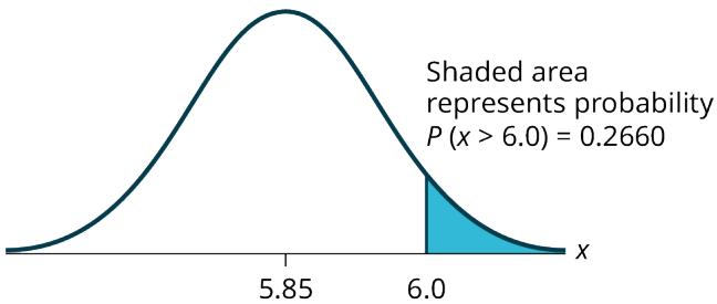
Figure 5.2.7 — The shaded right tail beyond a diameter of 6.0 cm. Its area is \(P(x > 6.0) = 0.2660\).
Part b — Split the leftover area between the tails.
$$ 1 - 0.20 = 0.80 $$The tails of the graph of the normal distribution each have an area of 0.40. Find \(k_1\), the \(40^{\text{th}}\) percentile, and \(k_2\), the \(60^{\text{th}}\) percentile, since \(0.40 + 0.20 = 0.60\).
$$ k_1 = \text{invNorm}(0.40, 5.85, 0.24) = 5.79\ \mathrm{cm} $$ $$ k_2 = \text{invNorm}(0.60, 5.85, 0.24) = 5.91\ \mathrm{cm} $$Part c — A percentile with an interpretation sentence.
$$ \text{invNorm}(0.90, 5.85, 0.24) = 6.16\ \mathrm{cm} $$Answer: a. \(P(x > 6.0) = 0.2660\); b. the middle 20% of mandarin oranges have diameters between 5.79 cm and 5.91 cm; c. the \(90^{\text{th}}\) percentile is 6.16 cm, so ninety percent of the mandarin oranges have a diameter of at most 6.16 cm.
Try it in rāSHio
Part b’s middle 20% is two inverse lookups, not one. In rāSHio choose Distributions → Normal, set mean 5.85 and standard deviation 0.24, then run Inverse (Left) at 0.40 and again at 0.60 to get the 5.79 cm and 5.91 cm edges — the two percentiles that leave 40% in each tail.
Problem Set 5.2
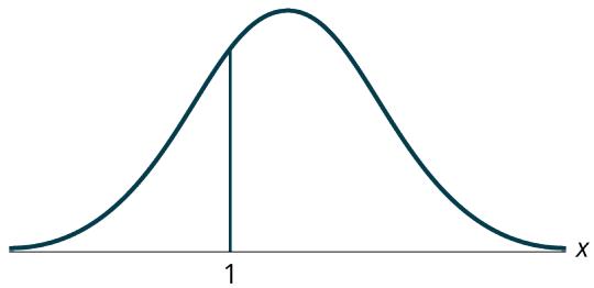
Problem 1. How would you represent the area to the left of one in a probability statement?
Solution
Step 1 — Name what the shading shows: the shaded region sits to the left of the value 1 on the \(x\)-axis, and area under a normal curve is probability.
Step 2 — Write it as a probability statement: "the area to the left of 1" is the probability that \(x\) lands below 1.
Answer: \(P(x < 1)\)
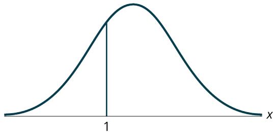
Problem 2. What is the area to the right of one?
Solution
Step 1 — Use the fact that the whole curve has area 1: the region to the left of 1 and the region to the right of 1 together fill the entire curve.
Step 2 — Subtract: the area to the right is whatever is left over after removing the area to the left.
$$ P(x > 1) = 1 - P(x < 1) $$Answer: The area to the right of one is \(1 - P(x < 1)\), which is the same thing as \(P(x > 1)\).
Problem 3. Is \(P(x < 1)\) equal to \(P(x \leq 1)\)? Why?
Solution
Step 1 — Ask what the two statements differ by: \(P(x \leq 1)\) includes the single point \(x = 1\); \(P(x < 1)\) does not.
Step 2 — Find the area of that single point: a single point on a continuous distribution has no width, so the region above it has no area.
$$ P(x = 1) = 0 $$Step 3 — Conclude: adding zero changes nothing.
Answer: Yes, they are equal, because in a continuous distribution \(P(x = 1) = 0\), so including or excluding the endpoint does not change the area.
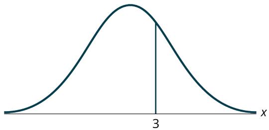
Problem 4. How would you represent the area to the left of three in a probability statement?
Solution
Step 1 — Read the shading: the region lies to the left of the value 3.
Answer: \(P(x < 3)\)
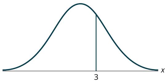
Problem 5. What is the area to the right of three?
Solution
Step 1 — Use the complement: the area to the right is the whole curve minus the area to the left.
$$ P(x > 3) = 1 - P(x < 3) $$Answer: The area to the right of three is \(1 - P(x < 3)\), which is the same thing as \(P(x > 3)\).
Problem 6. If the area to the left of \(x\) in a normal distribution is 0.123, what is the area to the right of \(x\)?
Solution
Step 1 — Subtract the left area from the total area of 1:
$$ 1 - 0.123 = 0.877 $$Answer: The area to the right of \(x\) is 0.877.
Problem 7. If the area to the right of \(x\) in a normal distribution is 0.543, what is the area to the left of \(x\)?
Solution
Step 1 — Subtract the right area from the total area of 1:
$$ 1 - 0.543 = 0.457 $$Answer: The area to the left of \(x\) is 0.457.
Use the following information to answer the next four exercises: \(X \sim N(54, 8)\).
Problem 8. Find the probability that \(x > 56\).
Solution
Step 1 — Identify the direction: the problem gives a value and asks for a probability, so this is a normalcdf question with the right tail shaded.
Step 2 — Set the bounds: the lower bound is 56 and the upper bound runs off the right end of the curve.
$$ P(x > 56) = \text{normalcdf}(56, 10^{99}, 54, 8) = 0.4013 $$Step 3 — Sanity-check: 56 is only a quarter of a standard deviation above the mean of 54, so a little under half the area should be to its right. It is.
Answer: \(P(x > 56) = 0.4013\)
Problem 9. Find the probability that \(x < 30\).
Solution
Step 1 — Identify the direction: a value is given and a probability is wanted, so use normalcdf with the left tail shaded.
Step 2 — Compute:
$$ P(x < 30) = \text{normalcdf}(-10^{99}, 30, 54, 8) = 0.0013 $$Step 3 — Sanity-check: \(z = \frac{30 - 54}{8} = -3\), so 30 sits three standard deviations below the mean, and the empirical rule says about 0.15% of the area is out past \(-3\). A value of 0.0013 is exactly that.
Answer: \(P(x < 30) = 0.0013\)
Problem 10. Find the \(80^{\text{th}}\) percentile.
Solution
Step 1 — Identify the direction: a percentile is asked for, so a probability goes in and a value comes out. That is invNorm.
Step 2 — Feed in the area to the left: the \(80^{\text{th}}\) percentile has 0.80 of the area below it.
$$ k = \text{invNorm}(0.80, 54, 8) = 60.73 $$Step 3 — Sanity-check: 0.80 is more than half, so \(k\) has to land above the mean of 54. It does.
Answer: The \(80^{\text{th}}\) percentile is 60.73, meaning 80% of the values are 60.73 or less.
Problem 11. Find the \(60^{\text{th}}\) percentile.
Solution
Step 1 — Run invNorm with the area to the left:
Answer: The \(60^{\text{th}}\) percentile is 56.03, meaning 60% of the values are 56.03 or less.
Problem 12. \(X \sim N(6, 2)\). Find the probability that \(x\) is between three and nine.
Solution
Step 1 — Recognize a between-question: both edges of the strip are given, so feed both to normalcdf.
Step 2 — Compute:
$$ P(3 < x < 9) = \text{normalcdf}(3, 9, 6, 2) = 0.8664 $$Step 3 — Sanity-check: three and nine sit exactly \(1.5\) standard deviations either side of the mean of six, so the strip should hold a bit less than the 95% that \(\pm 2\) standard deviations would. It does.
Answer: \(P(3 < x < 9) = 0.8664\)
Problem 13. \(X \sim N(-3, 4)\). Find the probability that \(x\) is between one and four.
Solution
Step 1 — Note that a negative mean changes nothing: the curve is centered at \(-3\) with a standard deviation of 4; the commands work the same way.
Step 2 — Compute:
$$ P(1 < x < 4) = \text{normalcdf}(1, 4, -3, 4) = 0.1186 $$Step 3 — Sanity-check: \(z = \frac{1-(-3)}{4} = 1\) and \(z = \frac{4-(-3)}{4} = 1.75\), so the strip lives entirely in the thin right shoulder of the curve. A small answer is expected.
Answer: \(P(1 < x < 4) = 0.1186\)
Problem 14. \(X \sim N(4, 5)\). Find the maximum of \(x\) in the bottom quartile.
Solution
Step 1 — Translate the words into an area: the bottom quartile is the lowest 25% of the values, so its maximum is the \(25^{\text{th}}\) percentile.
Step 2 — Run invNorm with an area to the left of 0.25:
Answer: The maximum of \(x\) in the bottom quartile is 0.63.
Use the following information to answer the next three exercises: The life of wearable fitness devices is normally distributed with a mean of 4.1 years and a standard deviation of 1.3 years. A wearable fitness device is guaranteed for three years. We are interested in the length of time a wearable fitness device lasts.
Problem 15. Find the probability that a wearable fitness device will break down during the guarantee period.
a) Sketch the situation. Label and scale the axes. Shade the region corresponding to the probability.
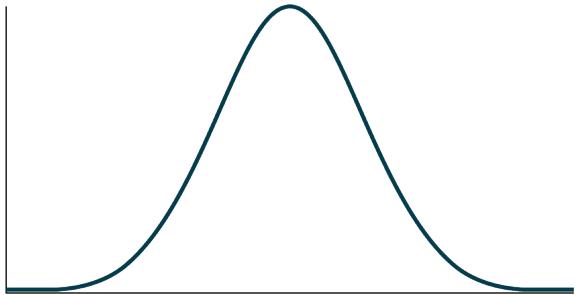
b) \(P(0 < x < \_\_\_\_) = \_\_\_\_\) (Use zero for the minimum value of \(x\).)
Solution
Step 1 — Set up (part a): let \(X\) = the life of a wearable fitness device in years, so \(X \sim N(4.1, 1.3)\). Draw a normal curve centered at 4.1, scale the axis in years, and shade everything from 0 out to 3. "Breaks down during the guarantee period" means the device fails before the three-year guarantee runs out.
Step 2 — Write the probability statement (part b): the problem tells you to use zero as the minimum value of \(x\), so the shaded strip runs from 0 to 3.
$$ P(0 < x < 3) = \text{normalcdf}(0, 3, 4.1, 1.3) = 0.1979 $$Answer: a. the shaded region runs from \(x = 0\) to \(x = 3\) on a curve centered at 4.1; b. \(P(0 < x < 3) = 0.1979\), so about 19.8% of these devices fail inside the guarantee period.
Problem 16. Find the probability that a wearable fitness device will last between 2.8 and six years.
a) Sketch the situation. Label and scale the axes. Shade the region corresponding to the probability.
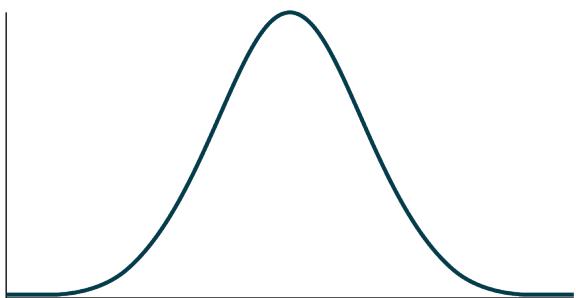
b) Write the probability statement and find the probability.
Solution
Step 1 — Sketch (part a): on the same \(N(4.1, 1.3)\) curve, shade the strip between \(x = 2.8\) and \(x = 6\). That strip straddles the mean, so it should hold most of the area.
Step 2 — Write and evaluate the probability statement (part b):
$$ P(2.8 < x < 6) = \text{normalcdf}(2.8, 6, 4.1, 1.3) = 0.7694 $$Answer: a. the shaded strip runs from 2.8 to 6 years; b. \(P(2.8 < x < 6) = 0.7694\).
Problem 17. Find the \(70^{\text{th}}\) percentile of the distribution for the time a wearable fitness device lasts.
a) Sketch the situation. Label and scale the axes. Shade the region corresponding to the lower 70%.
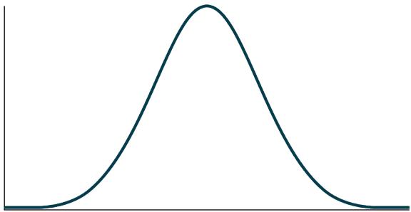
b) \(P(x < k) = \_\_\_\_\) Therefore, \(k = \_\_\_\_\)
Solution
Step 1 — Sketch (part a): shade the lower 70% of the area under the \(N(4.1, 1.3)\) curve. The boundary of that shading is the value you want.
Step 2 — Translate to a percentile (part b): the \(70^{\text{th}}\) percentile is the value \(k\) with \(P(x < k) = 0.70\).
$$ k = \text{invNorm}(0.70, 4.1, 1.3) = 4.78 $$Answer: a. the shading covers the lower 70% of the curve; b. \(P(x < k) = 0.70\), therefore \(k = 4.78\) years.
Use the following information to answer the next two exercises: The patient recovery time from a particular surgical procedure is normally distributed with a mean of 5.3 days and a standard deviation of 2.1 days.
Problem 18. What is the probability of spending more than two days in recovery?
a) 0.0580
b) 0.8447
c) 0.0553
d) 0.9420
Solution
Step 1 — Set up: let \(X\) = recovery time in days, so \(X \sim N(5.3, 2.1)\). "More than two days" is the area to the right of 2.
Step 2 — Compute:
$$ P(x > 2) = \text{normalcdf}(2, 10^{99}, 5.3, 2.1) = 0.9420 $$Step 3 — Check the distractor: 0.0580 is the area to the left of 2, which is what you get by shading the wrong side.
Answer: d. 0.9420
Problem 19. The \(90^{\text{th}}\) percentile for recovery times is?
a) 8.89
b) 7.07
c) 7.99
d) 4.32
Solution
Step 1 — Recognize a percentile: an area goes in and a number of days comes out, so use invNorm.
Step 2 — Compute:
$$ k = \text{invNorm}(0.90, 5.3, 2.1) = 7.99 $$Answer: c. 7.99
Use the following information to answer the next three exercises: The length of time it takes to find a parking space at 9 A.M. follows a normal distribution with a mean of five minutes and a standard deviation of two minutes.
Problem 20. Based upon the given information and numerically justified, would you be surprised if it took less than one minute to find a parking space?
a) Yes
b) No
c) Unable to determine
Solution
Step 1 — Set up: let \(X\) = the time in minutes to find a parking space, so \(X \sim N(5, 2)\).
Step 2 — Quantify how unusual one minute is:
$$ P(x < 1) = \text{normalcdf}(-10^{99}, 1, 5, 2) = 0.0228 $$Step 3 — Interpret: \(z = \frac{1 - 5}{2} = -2\), so one minute is two standard deviations below the mean, and only about 2.3% of mornings run that fast. Anything under about 5% is normally treated as surprising.
Answer: a. Yes. Only about 2.28% of the time does it take less than one minute, which is unusual enough to raise an eyebrow.
Problem 21. Find the probability that it takes at least eight minutes to find a parking space.
a) 0.0001
b) 0.9270
c) 0.1862
d) 0.0668
Solution
Step 1 — Translate "at least": at least eight minutes means \(x \geq 8\), the area to the right of 8.
Step 2 — Compute:
$$ P(x \geq 8) = \text{normalcdf}(8, 10^{99}, 5, 2) = 0.0668 $$Answer: d. 0.0668
Problem 22. Seventy percent of the time, it takes more than how many minutes to find a parking space?
a) 1.24
b) 2.41
c) 3.95
d) 6.05
Solution
Step 1 — Read the sentence carefully: "seventy percent of the time it takes MORE than \(k\) minutes" puts 0.70 of the area to the right of \(k\).
Step 2 — Convert to an area on the left, because invNorm only accepts a left-hand area.
Step 3 — Compute:
$$ k = \text{invNorm}(0.30, 5, 2) = 3.95 $$Step 4 — Sanity-check: the answer must be below the mean of five, since most of the time takes longer than it. It is.
Answer: c. 3.95
Problem 23. According to a study done by De Anza students, the height for Asian adult males is normally distributed with an average of 66 inches and a standard deviation of 2.5 inches. Suppose one Asian adult male is randomly chosen. Let \(X\) = height of the individual.
a) \(X \sim \_\_\_\_(\_\_\_\_, \_\_\_\_)\)
b) Find the probability that the person is between 65 and 69 inches. Include a sketch of the graph, and write a probability statement.
c) Would you expect to meet many Asian adult males over 72 inches? Explain why or why not, and justify your answer numerically.
Solution
Step 1 — State the distribution (part a): the mean is 66 inches and the standard deviation is 2.5 inches.
$$ X \sim N(66, 2.5) $$Step 2 — Find the between-probability (part b): sketch the curve centered at 66 and shade the strip from 65 to 69.
$$ P(65 < x < 69) = \text{normalcdf}(65, 69, 66, 2.5) = 0.5404 $$Step 3 — Judge the tail (part c):
$$ P(x > 72) = \text{normalcdf}(72, 10^{99}, 66, 2.5) = 0.0082 $$The value 72 is \(z = \frac{72 - 66}{2.5} = 2.4\) standard deviations above the mean, so fewer than 1 in 100 men in this group clear 72 inches.
Answer: a. \(X \sim N(66, 2.5)\); b. \(P(65 < x < 69) = 0.5404\); c. no, you would not expect to meet many, since the probability of exceeding 72 inches is only 0.0082, or about 0.8%.
Problem 24. IQ is normally distributed with a mean of 100 and a standard deviation of 15. Suppose one individual is randomly chosen. Let \(X\) = IQ of an individual.
a) \(X \sim \_\_\_\_(\_\_\_\_, \_\_\_\_)\)
b) Find the probability that the person has an IQ greater than 120. Include a sketch of the graph, and write a probability statement.
c) MENSA is an organization whose members have the top 2% of all IQs. Find the minimum IQ needed to qualify for the MENSA organization. Sketch the graph, and write the probability statement.
d) The middle 50% of IQs fall between what two values? Sketch the graph and write the probability statement.
Solution
Step 1 — State the distribution (part a):
$$ X \sim N(100, 15) $$Step 2 — Find the right tail (part b): shade everything above 120.
$$ P(x > 120) = \text{normalcdf}(120, 10^{99}, 100, 15) = 0.0912 $$Step 3 — Turn "top 2%" into a left-hand area (part c): if 2% is above the cutoff, then 98% is below it.
$$ 1 - 0.02 = 0.98 $$ $$ k = \text{invNorm}(0.98, 100, 15) = 130.81 $$The probability statement is \(P(x > k) = 0.02\), which is the same as \(P(x < k) = 0.98\).
Step 4 — Find the middle 50% (part d): the middle half runs from the first quartile to the third.
$$ Q_1 = \text{invNorm}(0.25, 100, 15) = 89.88 $$ $$ Q_3 = \text{invNorm}(0.75, 100, 15) = 110.12 $$The probability statement is \(P(89.88 < x < 110.12) = 0.50\).
Answer: a. \(X \sim N(100, 15)\); b. \(P(x > 120) = 0.0912\); c. an IQ of about 130.8 is the minimum needed for MENSA; d. the middle 50% of IQs fall between 89.88 and 110.12.
Problem 25. The percent of fat calories that a person in America consumes each day is normally distributed with a mean of about 36 and a standard deviation of 10. Suppose that one individual is randomly chosen. Let \(X\) = percent of fat calories.
a) \(X \sim \_\_\_\_(\_\_\_\_, \_\_\_\_)\)
b) Find the probability that the percent of fat calories a person consumes is more than 40. Graph the situation. Shade in the area to be determined.
c) Find the maximum number for the lower quarter of percent of fat calories. Sketch the graph and write the probability statement.
Solution
Step 1 — State the distribution (part a):
$$ X \sim N(36, 10) $$Step 2 — Shade the right tail (part b): shade everything above 40 on a curve centered at 36.
$$ P(x > 40) = \text{normalcdf}(40, 10^{99}, 36, 10) = 0.3446 $$Step 3 — Translate "lower quarter" (part c): the maximum of the lower quarter is the \(25^{\text{th}}\) percentile, so the probability statement is \(P(x < k) = 0.25\).
$$ k = \text{invNorm}(0.25, 36, 10) = 29.26 $$Answer: a. \(X \sim N(36, 10)\); b. \(P(x > 40) = 0.3446\); c. the maximum for the lower quarter is 29.26, so about 25% of people get less than 29.26% of their calories from fat.
Problem 26. Suppose that the distance of fly balls hit to the outfield (in baseball) is normally distributed with a mean of 250 feet and a standard deviation of 50 feet.
a) If \(X\) = distance in feet for a fly ball, then \(X \sim \_\_\_\_(\_\_\_\_, \_\_\_\_)\)
b) If one fly ball is randomly chosen from this distribution, what is the probability that this ball traveled fewer than 220 feet? Sketch the graph. Scale the horizontal axis \(X\). Shade the region corresponding to the probability. Find the probability.
c) Find the \(80^{\text{th}}\) percentile of the distribution of fly balls. Sketch the graph, and write the probability statement.
Solution
Step 1 — State the distribution (part a):
$$ X \sim N(250, 50) $$Step 2 — Shade the left tail (part b): on a horizontal axis scaled in feet and centered at 250, shade everything below 220.
$$ P(x < 220) = \text{normalcdf}(-10^{99}, 220, 250, 50) = 0.2743 $$Step 3 — Find the percentile (part c): the probability statement is \(P(x < k) = 0.80\).
$$ k = \text{invNorm}(0.80, 250, 50) = 292.08 $$Answer: a. \(X \sim N(250, 50)\); b. \(P(x < 220) = 0.2743\); c. the \(80^{\text{th}}\) percentile is 292.08 feet, so 80% of fly balls travel 292.08 feet or less.
Problem 27. In China, four-year-olds average three hours a day unsupervised. Most of the unsupervised children live in rural areas, considered safe. Suppose that the standard deviation is 1.5 hours and the amount of time spent alone is normally distributed. We randomly select one Chinese four-year-old living in a rural area. We are interested in the amount of time the child spends alone per day.
a) In words, define the random variable \(X\).
b) \(X \sim \_\_\_\_(\_\_\_\_, \_\_\_\_)\)
c) Find the probability that the child spends less than one hour per day unsupervised. Sketch the graph, and write the probability statement.
d) What percent of the children spend over ten hours per day unsupervised?
e) Seventy percent of the children spend at least how long per day unsupervised?
Solution
Step 1 — Define the variable (part a): \(X\) = the number of hours per day that a randomly selected rural Chinese four-year-old is unsupervised.
Step 2 — State the distribution (part b):
$$ X \sim N(3, 1.5) $$Step 3 — Shade the left tail (part c):
$$ P(x < 1) = \text{normalcdf}(-10^{99}, 1, 3, 1.5) = 0.0912 $$Step 4 — Shade the far right tail (part d):
$$ P(x > 10) = \text{normalcdf}(10, 10^{99}, 3, 1.5) < 0.0001 $$Ten hours is \(z = \frac{10 - 3}{1.5} \approx 4.67\) standard deviations above the mean, which is essentially off the end of the curve.
Step 5 — Convert the "at least" question (part e): 0.70 of the area sits to the right of \(k\), so \(1 - 0.70 = 0.30\) sits to the left.
$$ k = \text{invNorm}(0.30, 3, 1.5) = 2.21 $$Answer: a. \(X\) = hours per day a rural Chinese four-year-old spends unsupervised; b. \(X \sim N(3, 1.5)\); c. \(P(x < 1) = 0.0912\); d. less than 0.01% of the children; e. 2.21 hours.
Problem 28. In a certain presidential election, Alaska's 40 election districts averaged 1,956.8 votes per district for Candidate A. The standard deviation was 572.3. There are only 40 election districts in Alaska. The distribution of the votes per district for Candidate A was bell-shaped. Let \(X\) = number of votes for Candidate A for an election district.
a) State the approximate distribution of \(X\).
b) Is 1,956.8 a population mean or a sample mean? How do you know?
c) Find the probability that a randomly selected district had fewer than 1,600 votes for Candidate A. Sketch the graph and write the probability statement.
d) Find the probability that a randomly selected district had between 1,800 and 2,000 votes for Candidate A.
e) Find the third quartile for votes for Candidate A.
Solution
Step 1 — State the distribution (part a):
$$ X \sim N(1{,}956.8,\ 572.3) $$Step 2 — Decide population or sample (part b): Alaska has exactly 40 election districts and all 40 were used, so nothing was left out. A number computed from every member of the group is a population mean.
Step 3 — Shade the left tail (part c):
$$ P(x < 1{,}600) = \text{normalcdf}(-10^{99}, 1600, 1956.8, 572.3) = 0.2665 $$Step 4 — Shade the middle strip (part d):
$$ P(1{,}800 < x < 2{,}000) = \text{normalcdf}(1800, 2000, 1956.8, 572.3) = 0.1380 $$Step 5 — Find the third quartile (part e): \(Q_3\) is the \(75^{\text{th}}\) percentile.
$$ Q_3 = \text{invNorm}(0.75, 1956.8, 572.3) = 2{,}342.81 $$Answer: a. \(X \sim N(1{,}956.8,\ 572.3)\); b. a population mean, because every one of Alaska's 40 districts is included; c. \(P(x < 1{,}600) = 0.2665\); d. \(P(1{,}800 < x < 2{,}000) = 0.1380\); e. \(Q_3 = 2{,}342.81\) votes.
Problem 29. Suppose that the duration of a particular type of criminal trial is known to be normally distributed with a mean of 21 days and a standard deviation of seven days.
a) In words, define the random variable \(X\).
b) \(X \sim \_\_\_\_(\_\_\_\_, \_\_\_\_)\)
c) If one of the trials is randomly chosen, find the probability that it lasted at least 24 days. Sketch the graph and write the probability statement.
d) Sixty percent of all trials of this type are completed within how many days?
Solution
Step 1 — Define the variable (part a): \(X\) = the number of days a randomly chosen trial of this type lasts.
Step 2 — State the distribution (part b):
$$ X \sim N(21, 7) $$Step 3 — Translate "at least 24 days" (part c): at least 24 means \(x \geq 24\), the area to the right of 24.
$$ P(x \geq 24) = \text{normalcdf}(24, 10^{99}, 21, 7) = 0.3341 $$Step 4 — Translate "completed within" (part d): 60% finish at or below \(k\), so \(P(x < k) = 0.60\).
$$ k = \text{invNorm}(0.60, 21, 7) = 22.77 $$Answer: a. \(X\) = the duration in days of a randomly chosen trial; b. \(X \sim N(21, 7)\); c. \(P(x \geq 24) = 0.3341\); d. 60% of trials are completed within 22.77 days.
Problem 30. A motorcycle racer averages 129.71 seconds per 2.5 mile lap in a seven-lap race, with a standard deviation of 2.28 seconds. The distribution of their race times is normally distributed. We are interested in one of their randomly selected laps.
a) In words, define the random variable \(X\).
b) \(X \sim \_\_\_\_(\_\_\_\_, \_\_\_\_)\)
c) Find the percent of the racer's laps that are completed in less than 130 seconds.
d) The fastest 3% of the racer's laps are under ____.
e) The middle 80% of the racer's laps are from ____ seconds to ____ seconds.
Solution
Step 1 — Define the variable (part a): \(X\) = the time in seconds the racer takes to complete one randomly selected lap.
Step 2 — State the distribution (part b):
$$ X \sim N(129.71,\ 2.28) $$Step 3 — Shade the left tail (part c):
$$ P(x < 130) = \text{normalcdf}(-10^{99}, 130, 129.71, 2.28) = 0.5506 $$So about 55.06% of laps come in under 130 seconds.
Step 4 — Translate "fastest 3%" (part d): fastest means shortest, so those laps sit in the left tail and the area to the left is 0.03.
$$ k = \text{invNorm}(0.03, 129.71, 2.28) = 125.42 $$Step 5 — Translate "middle 80%" (part e): outside the middle 80% there is \(1 - 0.80 = 0.20\) of the area, split evenly into two tails of 0.10 each. The boundaries are therefore the \(10^{\text{th}}\) and \(90^{\text{th}}\) percentiles.
$$ k_1 = \text{invNorm}(0.10, 129.71, 2.28) = 126.79 $$ $$ k_2 = \text{invNorm}(0.90, 129.71, 2.28) = 132.63 $$Answer: a. \(X\) = lap time in seconds; b. \(X \sim N(129.71,\ 2.28)\); c. about 55.06%; d. the fastest 3% of laps are under 125.42 seconds; e. the middle 80% of laps run from 126.79 to 132.63 seconds.
Problem 31. Thuy Dau, Ngoc Bui, Sam Su, and Lan Voung conducted a survey as to how long customers at Lucky claimed to wait in the checkout line until their turn. Let \(X\) = time in line. Table 5.2.1 displays the ordered real data, in minutes.
| 0.50 | 4.25 | 5 | 6 | 7.25 |
| 1.75 | 4.25 | 5.25 | 6 | 7.25 |
| 2 | 4.25 | 5.25 | 6.25 | 7.25 |
| 2.25 | 4.25 | 5.5 | 6.25 | 7.75 |
| 2.25 | 4.5 | 5.5 | 6.5 | 8 |
| 2.5 | 4.75 | 5.5 | 6.5 | 8.25 |
| 2.75 | 4.75 | 5.75 | 6.5 | 9.5 |
| 3.25 | 4.75 | 5.75 | 6.75 | 9.5 |
| 3.75 | 5 | 6 | 6.75 | 9.75 |
| 3.75 | 5 | 6 | 6.75 | 10.75 |
a) Calculate the sample mean and the sample standard deviation.
b) Construct a histogram.
c) Draw a smooth curve through the midpoints of the tops of the bars.
d) In words, describe the shape of your histogram and smooth curve.
e) Let the sample mean approximate \(\mu\) and the sample standard deviation approximate \(\sigma\). The distribution of \(X\) can then be approximated by \(X \sim \_\_\_\_(\_\_\_\_, \_\_\_\_)\)
f) Use the distribution in part e to calculate the probability that a person will wait fewer than 6.1 minutes.
g) Determine the cumulative relative frequency for waiting less than 6.1 minutes.
h) Why aren't the answers to part f and part g exactly the same?
i) Why are the answers to part f and part g as close as they are?
j) If only ten customers had been surveyed rather than 50, do you think the answers to part f and part g would have been closer together or farther apart? Explain your conclusion.
Solution
Step 1 — Compute the sample statistics (part a): entering all 50 wait times into a list and running one-variable statistics gives
$$ \bar{x} = 5.51 \text{ minutes}, \qquad s = 2.15 \text{ minutes}. $$Step 2 — Build the histogram (part b): group the times into equal-width bins, for example one-minute bins from 0 to 11, and draw a bar over each bin whose height is the count of times falling in it. The tallest bars land in the 5-to-7 minute range, where most of the data sits.
Step 3 — Draw the smooth curve (part c): mark the midpoint of the top of each bar and connect the marks with one smooth line rather than a jagged path.
Step 4 — Describe the shape (part d): the curve rises from near zero at the left, peaks a bit past five minutes, and falls off with a slightly longer tail on the right. It is roughly bell-shaped and only mildly skewed right.
Step 5 — Approximate with a normal distribution (part e): using the sample mean for \(\mu\) and the sample standard deviation for \(\sigma\),
$$ X \sim N(5.51,\ 2.15). $$Step 6 — Use the model (part f):
$$ P(x < 6.1) = \text{normalcdf}(-10^{99}, 6.1, 5.51, 2.15) = 0.6083 $$Step 7 — Count the actual data (part g): 32 of the 50 recorded waits are shorter than 6.1 minutes.
$$ \frac{32}{50} = 0.64 $$Step 8 — Explain the gap (parts h, i, j): the two answers are not identical because the normal curve is only an approximation of the real distribution of waits, not a description of it. They are close because the sample has 50 values, and a normal approximation gets reliable once the sample size passes about 30. With only ten customers the two numbers would very likely be farther apart, since a smaller sample fits the smooth curve more loosely.
Answer: a. \(\bar{x} = 5.51\), \(s = 2.15\); e. \(X \sim N(5.51,\ 2.15)\); f. 0.6083; g. 0.64; h. the normal curve only approximates the real distribution; i. they agree closely because the sample size of 50 is comfortably above 30; j. farther apart, because a smaller sample matches the normal curve less well.
Problem 32. Suppose that Mateo and Anita attend different colleges. Mateo's GPA is the same as the average GPA at his school. Anita's GPA is 0.70 standard deviations above her school average. In complete sentences, explain why each of the following statements may be false.
a) Mateo's actual GPA is lower than Anita's actual GPA.
b) Mateo is not passing because his z-score is zero.
c) Anita is in the \(70^{\text{th}}\) percentile of students at her college.
Solution
Step 1 — Set up what is actually known: Mateo's \(z\)-score is 0 at his school, and Anita's \(z\)-score is 0.70 at hers. A \(z\)-score says where you stand relative to your own school, and nothing at all about the other school.
Step 2 — Test statement a: the two schools can have completely different average GPAs. If Mateo's school averages 3.4 and Anita's averages 2.5 with a standard deviation of 0.4, then Mateo's GPA is 3.4 and Anita's is \(2.5 + 0.70(0.4) = 2.78\). Mateo is higher, so the statement is false in that case.
Step 3 — Test statement b: a \(z\)-score of zero means exactly average for that school, not zero GPA. An average student at a school where the mean GPA is 3.0 has a 3.0 and is passing comfortably.
Step 4 — Test statement c: 0.70 standard deviations above the mean corresponds to an area to the left of \(P(z < 0.70) = 0.7580\), which is the \(75.8^{\text{th}}\) percentile, not the \(70^{\text{th}}\). The number of standard deviations and the percentile are different scales and only match by coincidence.
Answer: a. false whenever Mateo's school has a higher average than Anita's, since a \(z\)-score compares a student only to their own school; b. false because \(z = 0\) means average, not failing; c. false because 0.70 standard deviations above the mean is the \(75.8^{\text{th}}\) percentile, not the \(70^{\text{th}}\).
Problem 33. Table 5.2.2 shows a sample of the maximum capacity, meaning the maximum number of spectators, of sports stadiums. The table does not include horse-racing or motor-racing stadiums.
| 40,000 | 40,000 | 45,050 | 45,500 | 46,249 | 48,134 |
| 49,133 | 50,071 | 50,096 | 50,466 | 50,832 | 51,100 |
| 51,500 | 51,900 | 52,000 | 52,132 | 52,200 | 52,530 |
| 52,692 | 53,864 | 54,000 | 55,000 | 55,000 | 55,000 |
| 55,000 | 55,000 | 55,000 | 55,082 | 57,000 | 58,008 |
| 59,680 | 60,000 | 60,000 | 60,492 | 60,580 | 62,380 |
| 62,872 | 64,035 | 65,000 | 65,050 | 65,647 | 66,000 |
| 66,161 | 67,428 | 68,349 | 68,976 | 69,372 | 70,107 |
| 70,585 | 71,594 | 72,000 | 72,922 | 73,379 | 74,500 |
| 75,025 | 76,212 | 78,000 | 80,000 | 80,000 | 82,300 |
a) Calculate the sample mean and the sample standard deviation for the maximum capacity of sports stadiums.
b) Construct a histogram.
c) Draw a smooth curve through the midpoints of the tops of the bars of the histogram.
d) In words, describe the shape of your histogram and smooth curve.
e) Let the sample mean approximate \(\mu\) and the sample standard deviation approximate \(\sigma\). The distribution of \(X\) can then be approximated by \(X \sim \_\_\_\_(\_\_\_\_, \_\_\_\_)\)
f) Use the distribution in part e to calculate the probability that the maximum capacity of sports stadiums is less than 67,000 spectators.
g) Determine the cumulative relative frequency that the maximum capacity of sports stadiums is less than 67,000 spectators. Order the data and count the sports stadiums that have a maximum capacity less than 67,000, then divide by the total number of sports stadiums in the sample.
h) Why aren't the answers to part f and part g exactly the same?
Solution
Step 1 — Compute the sample statistics (part a): entering all 60 capacities and running one-variable statistics gives
$$ \bar{x} = 60{,}136, \qquad s = 10{,}468. $$Step 2 — Build the histogram (part b): use equal-width bins, for example 5,000-spectator bins running from 40,000 to 85,000, and draw a bar over each whose height is the number of stadiums in that range. The bars are tallest between 50,000 and 55,000.
Step 3 — Draw the smooth curve (part c): connect the midpoints of the bar tops with a single smooth line.
Step 4 — Describe the shape (part d): the curve climbs to a peak just above 50,000, then tapers off toward the largest stadiums. It is roughly bell-shaped with a mild right skew.
Step 5 — Approximate with a normal distribution (part e):
$$ X \sim N(60{,}136,\ 10{,}468) $$Step 6 — Use the model (part f):
$$ P(x < 67{,}000) = \text{normalcdf}(-10^{99}, 67000, 60136, 10468) = 0.7440 $$Step 7 — Count the actual data (part g): ordering the list and counting the stadiums below 67,000 gives 43 of the 60.
$$ \frac{43}{60} = 0.7167 $$Step 8 — Explain the gap (part h): the normal curve is a smooth model laid over data that is not exactly normal. The real data is slightly right-skewed and clumps heavily at round numbers like 55,000, so the model and the count disagree a little.
Answer: a. \(\bar{x} = 60{,}136\), \(s = 10{,}468\); e. \(X \sim N(60{,}136,\ 10{,}468)\); f. 0.7440; g. 0.7167; h. because the normal distribution only approximates this data, which is mildly right-skewed and clustered at round capacities.
Problem 34. An expert witness for a paternity lawsuit testifies that the length of a pregnancy is normally distributed with a mean of 280 days and a standard deviation of 13 days. The person who is being sued for lack of child support was out of the country from 240 to 306 days before the birth of the child, so the pregnancy would have been less than 240 days or more than 306 days long if he was the biological parent. The birth was uncomplicated, and the child needed no medical intervention. What is the probability that he was NOT the parent? What is the probability that he could be the parent? Calculate the z-scores first, and then use those to calculate the probability.
Solution
Step 1 — Set up: let \(X\) = the length of the pregnancy in days, so \(X \sim N(280, 13)\). He is not the parent exactly when the pregnancy would have been shorter than 240 days or longer than 306 days.
Step 2 — Compute both \(z\)-scores:
$$ z_1 = \frac{240 - 280}{13} = -3.08, \qquad z_2 = \frac{306 - 280}{13} = 2.00 $$Step 3 — Convert each to an area:
$$ P(x < 240) = P(z < -3.08) = 0.0010 $$ $$ P(x > 306) = P(z > 2.00) = 1 - 0.9772 = 0.0228 $$Step 4 — Add the two tails, because either one on its own rules him out.
$$ P(\text{not the parent}) = 0.0010 + 0.0228 = 0.0238 $$Step 5 — Take the complement for the other question:
$$ P(\text{could be the parent}) = 1 - 0.0238 = 0.9762 $$Answer: the probability that he was NOT the parent is 0.0238, and the probability that he could be the parent is 0.9762.
Problem 35. An automotive factory can build an average of 6,000 cars and trucks a week. Generally, 10% of the cars were defective coming off the assembly line. Suppose we draw a random sample of \(n = 100\) cars. Let \(X\) represent the number of defective cars in the sample. What can we say about \(X\) in regard to the 68-95-99.7 empirical rule, meaning one standard deviation, two standard deviations, and three standard deviations from the mean? Assume a normal distribution for the defective cars in the sample.
Solution
Step 1 — Read off the parameters: \(n = 100\), \(p = 0.1\), \(q = 1 - p = 0.9\).
Step 2 — Compute the mean and standard deviation:
$$ \mu = np = (100)(0.10) = 10 $$ $$ \sigma = \sqrt{npq} = \sqrt{(100)(0.1)(0.9)} = 3 $$Step 3 — Step out one standard deviation:
$$ x_1 = \mu + z\sigma = 10 + 1(3) = 13, \qquad x_2 = \mu - z\sigma = 10 - 1(3) = 7 $$About 68% of samples will have between seven and 13 defective cars.
Step 4 — Step out two standard deviations:
$$ x_1 = 10 + 2(3) = 16, \qquad x_2 = 10 - 2(3) = 4 $$About 95% of samples will have between four and 16 defective cars.
Step 5 — Step out three standard deviations:
$$ x_1 = 10 + 3(3) = 19, \qquad x_2 = 10 - 3(3) = 1 $$About 99.7% of samples will have between one and 19 defective cars.
Answer: with \(\mu = 10\) and \(\sigma = 3\): 68% of samples fall between seven and 13 defective cars, 95% between four and 16, and 99.7% between one and 19.
Problem 36. We flip a coin 100 times \((n = 100)\) and note that it only comes up heads 20% \((p = 0.20)\) of the time. The mean and standard deviation for the number of times the coin lands on heads is \(\mu = 20\) and \(\sigma = 4\). Verify the mean and standard deviation, then solve the following.
a) There is about a 68% chance that the number of heads will be somewhere between ____ and ____.
b) There is about a ____ chance that the number of heads will be somewhere between 12 and 28.
c) There is about a ____ chance that the number of heads will be somewhere between eight and 32.
Solution
Step 1 — Verify the mean and standard deviation: with \(n = 100\), \(p = 0.20\), and \(q = 0.80\),
$$ \mu = np = (100)(0.20) = 20 $$ $$ \sigma = \sqrt{npq} = \sqrt{(100)(0.20)(0.80)} = \sqrt{16} = 4 $$Both match the values given.
Step 2 — Apply the 68% band (part a): one standard deviation either side of the mean runs from \(20 - 4 = 16\) to \(20 + 4 = 24\).
Step 3 — Recognize the 12-to-28 band (part b): \(12 = 20 - 2(4)\) and \(28 = 20 + 2(4)\), so this is two standard deviations either side, which is about 95%.
Step 4 — Recognize the 8-to-32 band (part c): \(8 = 20 - 3(4)\) and \(32 = 20 + 3(4)\), so this is three standard deviations either side, which is about 99.7%.
Answer: a. between 16 and 24; b. about a 95% chance; c. about a 99.7% chance.
Problem 37. A $1 scratch off lotto ticket will be a winner one out of five times. Out of a shipment of \(n = 190\) lotto tickets, find the probability for the lotto tickets that there are
a) somewhere between 34 and 54 prizes.
b) somewhere between 54 and 64 prizes.
c) more than 64 prizes.
Solution
Step 1 — Read off the parameters: \(n = 190\) and \(p = \frac{1}{5} = 0.2\), so \(q = 0.8\).
Step 2 — Compute the mean and standard deviation:
$$ \mu = np = (190)(0.2) = 38 $$ $$ \sigma = \sqrt{npq} = \sqrt{(190)(0.2)(0.8)} = \sqrt{30.4} = 5.5136 $$Step 3 — Find the middle strip (part a):
$$ P(34 < x < 54) = \text{normalcdf}(34, 54, 38, 5.5136) = 0.7641 $$Step 4 — Find the upper strip (part b):
$$ P(54 < x < 64) = \text{normalcdf}(54, 64, 38, 5.5136) = 0.0019 $$Both 54 and 64 sit far out in the right tail, so almost no area is left between them.
Step 5 — Find the far right tail (part c):
$$ P(x > 64) = \text{normalcdf}(64, 10^{99}, 38, 5.5136) = 0.0000012 $$That is \(z = \frac{64 - 38}{5.5136} \approx 4.7\) standard deviations above the mean, which is effectively impossible.
Answer: a. 0.7641; b. 0.0019; c. 0.0000012, approximately zero.
Problem 38. On average, 28% of 18 to 34 year olds check social media before getting out of bed in the morning. Suppose this percentage follows a normal distribution with a standard deviation of 5%.
a) Find the probability that the percent of 18 to 34-year-olds who check social media before getting out of bed in the morning is at least 30.
b) Find the \(95^{\text{th}}\) percentile, and express it in a sentence.
Solution
Step 1 — Set up: let \(X\) = the percent of 18-to-34 year olds who check social media before getting out of bed, so \(X \sim N(28, 5)\).
Step 2 — Translate "at least 30" (part a): at least 30 means \(x \geq 30\), the area to the right of 30.
$$ P(x \geq 30) = \text{normalcdf}(30, 10^{99}, 28, 5) = 0.3446 $$Step 3 — Find the percentile (part b):
$$ k = \text{invNorm}(0.95, 28, 5) = 36.22 $$Answer: a. \(P(x \geq 30) = 0.3446\); b. the \(95^{\text{th}}\) percentile is 36.22, which means that 95% of the time no more than about 36.2% of 18-to-34 year olds check social media before getting out of bed.
Key Terms
percentile — the value \(k\) with a stated percent of the distribution at or below it; the \(p^{\text{th}}\) percentile satisfies \(P(X < k) = p/100\).
critical value — a value on the \(x\)-axis that splits a distribution into a specified area to its left and the rest to its right.
normalcdf — the calculator command that takes a lower bound, an upper bound, a mean, and a standard deviation, and returns the area between the bounds.
invNorm — the calculator command that takes an area to the left, a mean, and a standard deviation, and returns the value \(k\) at that percentile.