8.3 Transformations for Skewed Data
County population size among the counties in the US is very strongly right skewed. Can we apply a transformation to make the distribution more symmetric? How would such a transformation affect the scatterplot and residual plot when another variable is graphed against this variable? In this section, we will see the power of transformations for very skewed data.
Most of the data you meet in a first statistics course is bell-shaped or close to it, but the real world is full of variables that are not. County populations, household incomes, insurance claim sizes, earthquake magnitudes, and city sizes are all famously right-skewed: a huge pile of small values and a long thin tail of very large ones. Plain linear regression assumes the spread of points around the line is roughly constant and that the relationship is roughly linear — both assumptions that skewed data routinely violate. Transformations are the standard fix: we rescale the variable so its distribution looks more symmetric, and the regression tools we built in Sections 8.1 and 8.2 suddenly work again.
A transformation is just a new set of axis labels. We do not change the data — we change the ruler we use to measure it. The \(\log_{10}\) transformation, for example, relabels "10" as 1, "100" as 2, "1,000" as 3, "10,000" as 4, and so on. Every factor of 10 gets the same amount of axis space. Distances that used to be compressed into a corner of the plot are now spread out, and tiny wiggles that were invisible become clearly visible. Nothing about the underlying counties, trucks, or incomes has changed — we are just looking at them through a different lens.
Learning Objectives
Source: Main Text
By the end of this section, you should be able to:
- See how a log transformation can bring symmetry to an extremely skewed variable.
- Recognize that data can often be transformed to produce a linear relationship, and that this transformation often involves log of the \(y\)-values and sometimes log of the \(x\)-values.
- Use residual plots to assess whether a linear model for transformed data is reasonable.
8.3.1 Transformations to Reduce Skew
Source: Main Text
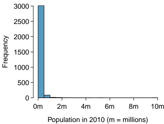
Consider the histogram of county populations shown in Figure 8.22(a), which shows extreme skew. What isn't useful about this plot?
Solution
Nearly all of the data fall into the left-most bin, and the extreme skew obscures many of the potentially interesting details in the data.
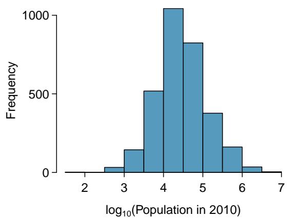
There are some standard transformations that may be useful for strongly right-skewed data where much of the data is positive but clustered near zero. A transformation is a rescaling of the data using a function. For instance, a plot of the logarithm (base 10) of county populations results in the new histogram in Figure 8.22(b). This data is symmetric, and any potential outliers appear much less extreme than in the original data set. By reining in the outliers and extreme skew, transformations like this often make it easier to build statistical models against the data.
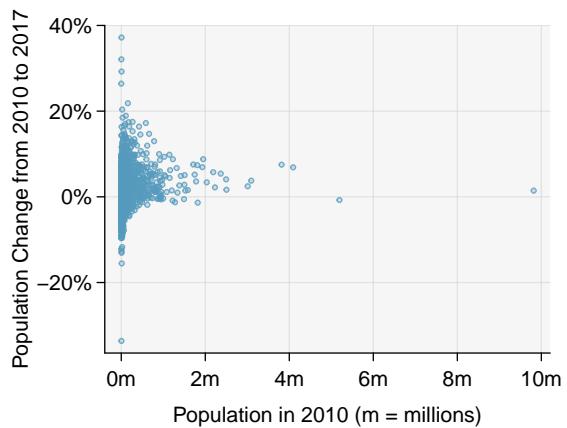
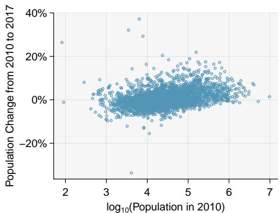
Transformations can also be applied to one or both variables in a scatterplot. A scatterplot of the population change from 2010 to 2017 against the population in 2010 is shown in Figure 8.23(a). In this first scatterplot, it's hard to decipher any interesting patterns because the population variable is so strongly skewed. However, if we apply a \(\log_{10}\) transformation to the population variable, as shown in Figure 8.23(b), a positive association between the variables is revealed. While fitting a line to predict population change (2010 to 2017) from population (in 2010) does not seem reasonable, fitting a line to predict population change from \(\log_{10}(\text{population})\) does seem reasonable.
Transformations other than the logarithm can be useful, too. For instance, the square root (\(\sqrt{\text{original observation}}\)) and inverse (\(\frac{1}{\text{original observation}}\)) are commonly used by data scientists. Common goals in transforming data are to see the data structure differently, reduce skew, assist in modeling, or straighten a nonlinear relationship in a scatterplot.
(a)
(b)
Figure 8.22: (a) A histogram of the populations of all US counties. (b) A histogram of \(\log_{10}\)-transformed county populations. For this plot, the x-value corresponds to the power of 10, e.g. "4" on the x-axis corresponds to \(10^{4} = 10{,}000\).
(a)
(b)
Figure 8.23: (a) Scatterplot of population change against the population before the change. (b) A scatterplot of the same data but where the population size has been log-transformed.
Common Transformations for Right-Skewed Data
Three transformations show up over and over again when a variable is positive and right-skewed:
- Log transformation, \(x \mapsto \log_{10}(x)\) or \(x \mapsto \ln(x)\): compresses large values heavily, leaves small values roughly alone. This is the workhorse.
- Square root, \(x \mapsto \sqrt{x}\): milder compression than the log. Often used for counts (number of events in a fixed time window).
- Inverse, \(x \mapsto 1/x\): very aggressive compression of large values. Sometimes used when rates or reciprocals are the natural quantity.
The goal in every case is the same: produce a distribution (or scatterplot) that is more symmetric, more linear, and better suited to the tools we already have.
Source: Main Text
The following ten hypothetical county populations (rounded, in thousands) are strongly right-skewed:
\(\{5, 8, 12, 15, 20, 40, 80, 200, 900, 5000\}\)
(a) By eye, describe the shape of the distribution of the raw counts. (b) Apply the \(\log_{10}\) transformation to each value. (You may round to two decimals.) (c) Describe the shape of the transformed distribution — is it more symmetric than the original?
Solution
(a) Strongly right-skewed: most values are small (between 5 and 40) and there is a long tail of large values (200, 900, 5000). The mean is pulled far to the right of the median by the big values.
(b) Taking \(\log_{10}\) of each (populations in thousands):
| Raw \(x\) | \(\log_{10}(x)\) |
|---|---|
| 5 | 0.70 |
| 8 | 0.90 |
| 12 | 1.08 |
| 15 | 1.18 |
| 20 | 1.30 |
| 40 | 1.60 |
| 80 | 1.90 |
| 200 | 2.30 |
| 900 | 2.95 |
| 5000 | 3.70 |
(c) Much more symmetric. The raw range is 5 to 5000 (three orders of magnitude); the transformed range is 0.70 to 3.70 (three units on the \(\log_{10}\) scale). The values now spread out evenly instead of piling up at the small end, so the distribution looks roughly bell-shaped rather than severely right-skewed.
8.3.2 Transformations to Achieve Linearity
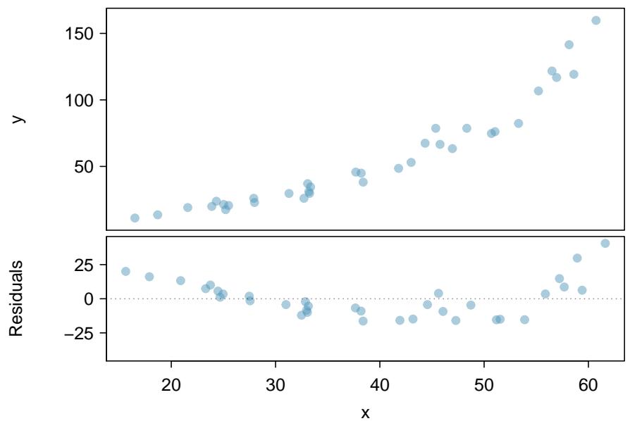
Figure 8.24: Variable \(y\) is plotted against \(x\). A nonlinear relationship is evident by the \(\cup\)-pattern shown in the residual plot. The curvature is also visible in the original plot.
Source: Main Text
Consider the scatterplot and residual plot in Figure 8.24. The regression output is also provided. Is the linear model \(\hat{y} = -52.3564 + 2.7842 x\) a good model for the data?
Solution
The regression equation is
$$ \hat{y} = -52.3564 + 2.7842 x $$| Predictor | Coef | SE Coef | T | P |
|---|---|---|---|---|
| Constant | -52.3564 | 7.2757 | -7.196 | 3e-08 |
| x | 2.7842 | 0.1768 | 15.752 | \(< 2\)e-16 |
\(S = 13.76\), \(R\)-Sq \(= 88.26\%\), \(R\)-Sq(adj) \(= 87.91\%\).
We can note the \(R^{2}\) value is fairly large. However, this alone does not mean that the model is good. Another model might be much better. When assessing the appropriateness of a linear model, we should look at the residual plot. The \(\cup\)-pattern in the residual plot tells us the original data is curved. If we inspect the two plots, we can see that for small and large values of \(x\) we systematically underestimate \(y\), whereas for middle values of \(x\), we systematically overestimate \(y\). The curved trend can also be seen in the original scatterplot. Because of this, the linear model is not appropriate, and it would not be appropriate to perform a \(t\)-test for the slope because the conditions for inference are not met. However, we might be able to use a transformation to linearize the data.
Regression analysis is easier to perform on linear data. When data are nonlinear, we sometimes transform the data in a way that makes the resulting relationship linear. The most common transformation is log of the \(y\)-values. Sometimes we also apply a transformation to the \(x\)-values. We generally use the residuals as a way to evaluate whether the transformed data are more linear. If so, we can say that a better model has been found.
Source: Main Text
Using the regression output for the transformed data, write the new linear regression equation.
Solution
The regression equation is
$$ \widehat{\log(y)} = 1.722540 + 0.052985 x $$| Predictor | Coef | SE Coef | T | P |
|---|---|---|---|---|
| Constant | 1.722540 | 0.056731 | 30.36 | \(< 2\)e-16 |
| x | 0.052985 | 0.001378 | 38.45 | \(< 2\)e-16 |
The linear regression equation can be written as: \(\widehat{\log(y)} = 1.723 + 0.053 x\).
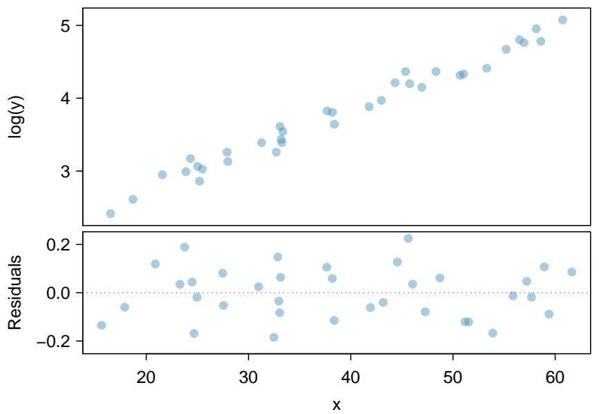
Figure 8.25: A plot of \(\log(y)\) against \(x\). The residuals don't show any evident patterns, which suggests the transformed data is well-fit by a linear model.
Source: Main Text
Compute the \(95\%\) confidence interval for the family income coefficient using the regression output from Table 8.21.
Solution
The point estimate is \(-0.0431\) and the standard error is \(SE = 0.0108\). When constructing a confidence interval for a model coefficient, we generally use a \(t\)-distribution. The degrees of freedom for the distribution are noted in the regression output, \(df = 48\), allowing us to identify \(t_{48}^{\star} = 2.01\) for use in the confidence interval.
We can now construct the confidence interval in the usual way:
$$ \text{point estimate} \pm t_{48}^{\star} \times SE \quad \rightarrow \quad -0.0431 \pm 2.01 \times 0.0108 \quad \rightarrow \quad (-0.0648,\ -0.0214) $$We are \(95\%\) confident that with each dollar increase in family income, the university's gift aid is predicted to decrease on average by \$0.0214 to \$0.0648.
Source: Main Text
Which of the following statements are true? There may be more than one.
(a) There is an apparent linear relationship between \(x\) and \(y\).
(b) There is an apparent linear relationship between \(x\) and \(\widehat{\log(y)}\).
(c) The model provided by Regression I \((\hat{y} = -52.3564 + 2.7842 x)\) yields a better fit.
(d) The model provided by Regression II \((\widehat{\log(y)} = 1.723 + 0.053 x)\) yields a better fit.
Solution
True statements: (b) and (d).
(a) False. The original scatterplot shows clear curvature, and the residual plot in Figure 8.24 shows a \(\cup\)-pattern — strong evidence that \(x\) and \(y\) are not linearly related.
(b) True. After applying the log transformation to \(y\), the residuals in Figure 8.25 show no pattern, which is the diagnostic for a good linear fit. The scatterplot of \(\log(y)\) versus \(x\) also looks linear.
(c) False. Regression I has \(R^{2} = 88.26\%\), but the curved residual pattern invalidates it — the high \(R^{2}\) is misleading because the model is fundamentally the wrong shape.
(d) True. Regression II has \(R^{2} = 97.82\%\) and a clean residual plot. Both indicators agree: the log-transformed model is a much better fit.
The pattern in residuals always trumps a single summary statistic like \(R^{2}\). A model with smaller \(R^{2}\) but clean residuals is almost always better than one with larger \(R^{2}\) but systematic residual patterns.
When you find a curve in a residual plot, your first question should be what transformation might straighten it? For right-skewed \(x\), try \(\log(x)\). For exponential growth or decay in \(y\), try \(\log(y)\). For data that bends like a square root, try \(\sqrt{y}\). There is no universal recipe — you try a transformation, make a new residual plot, and check whether the pattern has disappeared. If it has, you have earned the right to use linear regression on the transformed data. If not, try a different transformation or accept that a nonlinear model is needed.
The phrase "a better model has been found" deserves a caveat: a model on \(\log(y)\) is a different model than a model on \(y\). The slope in Regression II tells us how \(\log(y)\) changes with \(x\), which translates to a multiplicative change in \(y\) itself — each unit increase in \(x\) multiplies \(y\) by roughly \(10^{0.053} \approx 1.13\), i.e., a \(13\%\) increase per unit. Interpreting a log-linear regression line means keeping that multiplicative story straight. We will see this again when we interpret slopes in the exercises at the end of this section.
Source: Main Text
A researcher fits a regression of \(y\) on \(x\) for 50 observations and gets \(R^{2} = 0.92\), a large slope \(t\)-statistic, and a residual plot that has a clear \(\cap\)-shape (down-then-up inverted bowl).
(a) Based on \(R^{2}\) alone, does the linear model look good? (b) Based on the residual plot, should we trust the linear model? (c) What is one thing the researcher should try before reporting the results of the regression?
Solution
(a) Yes — \(R^{2} = 0.92\) means the linear model explains \(92\%\) of the variability in \(y\). Taken alone, this looks like a strong fit.
(b) No. The \(\cap\)-pattern in the residual plot means the model is systematically wrong: it overestimates \(y\) at the extremes and underestimates \(y\) in the middle (or vice versa, depending on sign). Systematic error is exactly what a linear model is not supposed to have. The \(R^{2}\) is misleading because the model is the wrong shape, not because it is noisy.
(c) Try a transformation. A \(\cap\)-shape often suggests taking \(\log(y)\) (or \(\sqrt{y}\)) to flatten the curve, or transforming \(x\) (e.g., \(x \mapsto x^{2}\) or \(x \mapsto \log(x)\)) to straighten the underlying relationship. After the transformation, make a new residual plot: if it looks like random static, the transformed model is a better fit. Only report the transformed model if the residuals support it.
Section Summary
- A transformation is a rescaling of the data using a function. When data are very skewed, a log transformation often results in more symmetric data.
- Regression analysis is easier to perform on linear data. When data are nonlinear, we sometimes transform the data in a way that results in a linear relationship. The most common transformation is log of the \(y\)-values. Sometimes we also apply a transformation to the \(x\)-values.
- To assess the model, we look at the residual plot of the transformed data. If the residual plot of the original data has a pattern, but the residual plot of the transformed data has no pattern, a linear model for the transformed data is reasonable, and the transformed model provides a better fit than the simple linear model.
- \(R^{2}\) alone is not enough to judge a model. A high \(R^{2}\) with a patterned residual plot still indicates a poor fit. Always make the residual plot.
Problem Set
Source: Main Text
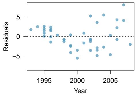
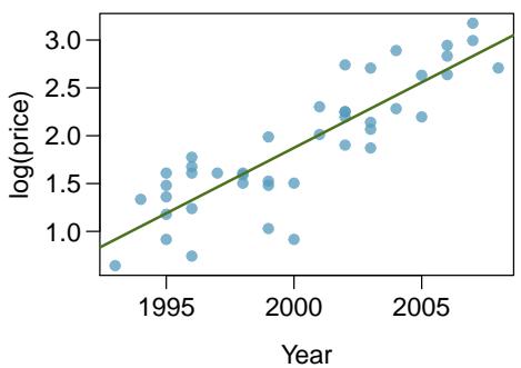
Problem 1: Used trucks. The scatterplot below shows the relationship between year and price (in thousands of dollars) of a random sample of 42 pickup trucks. Also shown is a residuals plot for the linear model for predicting price from year.
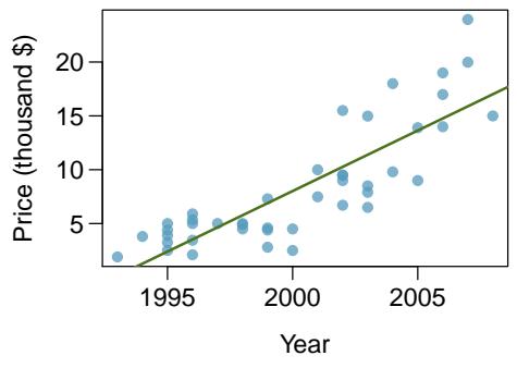
(a) Describe the relationship between these two variables and comment on whether a linear model is appropriate for modeling the relationship between year and price.
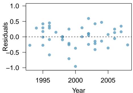
(b) The scatterplot below shows the relationship between logged (natural log) price and year of these trucks, as well as the residuals plot for modeling these data. Comment on which model (linear model from earlier or logged model presented here) is a better fit for these data.
(c) The output for the logged model is given below. Interpret the slope in context of the data.
| Estimate | Std. Error | t value | Pr(>\ | t\ | ) | |
|---|---|---|---|---|---|---|
| (Intercept) | -271.981 | 25.042 | -10.861 | 0.000 | ||
| Year | 0.137 | 0.013 | 10.937 | 0.000 |
Problem 8.31 Solution
Part (a) — Assess the original linear model.
The scatterplot of truck price versus year shows a curved, nonlinear relationship: prices stay low and flat for older trucks, then rise sharply (accelerating) for more recent years. The residual plot for the linear fit reveals this clearly — there is a pronounced \(\cup\)-shape: residuals are positive for very old and very new trucks and negative for middle-aged trucks. A curved residual pattern means the linear model systematically under- or over-predicts in a nonrandom way, so a simple linear model is not appropriate for these data.
Part (b) — Compare linear vs. log-transformed model.
After transforming price with the natural log, the relationship between \(\ln(\text{price})\) and year looks much closer to linear, and the residual plot loses its clear \(\cup\)-pattern — residuals are scattered randomly around zero with roughly constant spread. Because the residual plot for the log-transformed model has no obvious pattern while the original does, the logged model is a better fit for the data.
Part (c) — Interpret the slope in context.
The logged model is \(\widehat{\ln(\text{price})} = -271.981 + 0.137 \cdot \text{Year}\). The slope is \(0.137\) on the log scale, so each additional year of the truck's model year is associated with a \(0.137\) increase in \(\ln(\text{price})\). On the original price scale this is a multiplicative change: \(e^{0.137} \approx 1.147\). Each additional model year is associated with roughly a \(14.7\%\) increase in predicted price (in thousands of dollars), on average.
In context: holding all else constant, a pickup truck that is one model year newer is predicted to be priced about \(14.7\%\) higher.
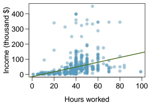
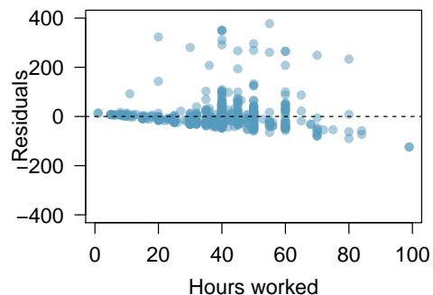
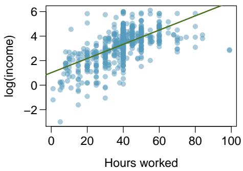
Problem 2: Income and hours worked. The scatterplot below shows the relationship between income and years worked for a random sample of 787 Americans. Also shown is a residuals plot for the linear model for predicting income from hours worked. The data come from the 2012 American Community Survey.
(a) Describe the relationship between these two variables and comment on whether a linear model is appropriate for modeling the relationship between year and price.
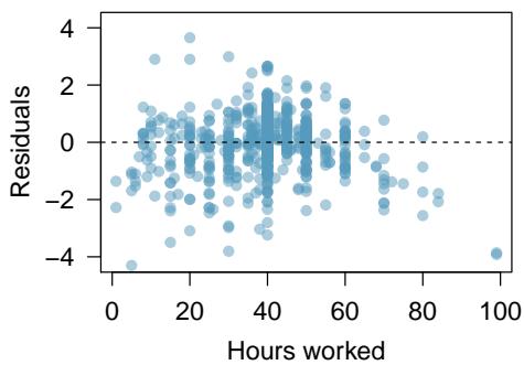
(b) The scatterplot below shows the relationship between logged (natural log) income and hours worked, as well as the residuals plot for modeling these data. Comment on which model (linear model from earlier or logged model presented here) is a better fit for these data.
(c) The output for the logged model is given below. Interpret the slope in context of the data.
| Estimate | Std. Error | t value | Pr(>\ | t\ | ) | |
|---|---|---|---|---|---|---|
| (Intercept) | 1.017 | 0.113 | 9.000 | 0.000 | ||
| hrs_work | 0.058 | 0.003 | 21.086 | 0.000 |
Problem 8.32 Solution
Part (a) — Assess the original linear model.
The scatterplot of income versus hours worked shows a weak, fan-shaped pattern: income generally increases with hours worked, but the spread in income grows dramatically as hours worked increases. The residual plot confirms this — residuals are small for small values of hours worked and become very large (both positive and far positive) for larger values, producing a clear fan or funnel shape. This violates the "constant variability" condition for linear regression. A simple linear model is not appropriate for these data.
Part (b) — Compare linear vs. log-transformed model.
After applying the natural log transformation to income, the relationship between \(\ln(\text{income})\) and hours worked is more linear and, importantly, the residual plot for the logged model shows residuals scattered around zero with roughly constant spread — the fan pattern is largely gone. Because the log-transformed model has cleaner residuals (no pattern, constant variability), the logged model is a better fit than the original linear model.
Part (c) — Interpret the slope in context.
The logged model is \(\widehat{\ln(\text{income})} = 1.017 + 0.058 \cdot \text{hrs\_work}\). The slope \(0.058\) is on the log scale, so each additional hour worked per week is associated with a \(0.058\) increase in \(\ln(\text{income})\). On the original income scale this corresponds to multiplying income by \(e^{0.058} \approx 1.060\). Each additional hour worked is associated with roughly a \(6.0\%\) increase in predicted income, on average.
In context: for a random American in this 2012 sample, working one additional hour per week is associated with a predicted income that is about \(6\%\) higher.