8.4 Inference for the Slope of a Regression Line
Here we encounter our last confidence interval and hypothesis test procedures, this time for making inferences about the slope of the population regression line. We can use these tools to answer questions such as:
- Is the unemployment rate a significant linear predictor for the loss of the President's party in the House of Representatives?
- On average, how much less in college gift aid do students receive when their parents earn an additional \$1,000 in income?
Until now, the regression line has been a description — a best-fit line drawn through the data we actually collected. But the points we have are just one sample from a much larger population of possible observations. The slope we computed could have come out a bit higher or a bit lower if we had sampled different people. Slope inference is how we turn "the line we drew" into a statement about "the line that lives in the population" — confidence intervals give us a plausible range for the true slope, and hypothesis tests let us decide whether the true slope could be zero.
If you can run a \(t\)-test for a mean, you can run a \(t\)-test for a slope. The machinery is identical: point estimate, standard error, degrees of freedom, \(t\)-statistic, p-value. The only new thing is where the numbers come from — you read them off a regression output table instead of computing \(\bar{x}\) and \(s\) by hand.
Learning Objectives
Source: Main Text
By the end of this section, you should be able to:
- Recognize that the slope of the sample regression line is a point estimate and has an associated standard error.
- Read the results of computer regression output and identify the quantities needed for inference for the slope of the regression line — specifically the slope of the sample regression line, the SE of the slope, and the degrees of freedom.
- State and verify whether the conditions are met for inference on the slope of the regression line using the \(t\)-distribution.
- Carry out a complete confidence interval procedure for the slope of the regression line.
- Carry out a complete hypothesis test for the slope of the regression line.
- Distinguish between when to use the \(t\)-test for the slope of a regression line and when to use the one-sample \(t\)-test for a mean of differences.
8.4.1 The Role of Inference for Regression Parameters
Previously, we found the equation of the regression line for predicting gift aid from family income at Elmhurst College. The slope, \(b\), was equal to \(-0.0431\). This is the slope for our sample data. However, the sample was taken from a larger population. We would like to use the slope computed from our sample data to estimate the slope of the population regression line.
The equation for the population regression line can be written as
$$ \mu_y = \alpha + \beta x $$Here, \(\alpha\) and \(\beta\) represent two model parameters — the \(y\)-intercept and the slope of the true (population) regression line. (This use of \(\alpha\) and \(\beta\) has nothing to do with the \(\alpha\) and \(\beta\) we used previously to represent the probabilities of Type I and Type II errors!) The parameters \(\alpha\) and \(\beta\) are estimated using data. We can look at the equation of the regression line calculated from a particular data set:
$$ \hat{y} = a + b x $$and see that \(a\) and \(b\) are point estimates for \(\alpha\) and \(\beta\), respectively. If we plug in the values of \(a\) and \(b\), the regression equation for predicting gift aid based on family income is:
$$ \hat{y} = 24{.}3193 - 0{.}0431 x $$The slope of the sample regression line, \(-0.0431\), is our best estimate for the slope of the population regression line, but there is variability in this estimate since it is based on a sample. A different sample would produce a somewhat different estimate of the slope. The standard error of the slope tells us the typical variation in the slope of the sample regression line and the typical error in using this slope to estimate the slope of the population regression line.
We would like to construct a 95% confidence interval for \(\beta\), the slope of the population regression line. As with means, inference for the slope of a regression line is based on the \(t\)-distribution.
The leap from \(b\) to \(\beta\) is the same leap you've been making all along — from \(\bar{x}\) to \(\mu\), from \(\hat{p}\) to \(p\). Sample statistic to population parameter. The slope is just another statistic that wobbles from sample to sample, and \(\beta\) is the fixed (but unknown) quantity we'd love to pin down.
Source: Main Text
The intercept and slope estimates for the Elmhurst data are \(b_0 = 24{,}319\) and \(b_1 = -0.0431\). What do these numbers really mean?
Solution
Interpreting the slope parameter is helpful in almost any application. For each additional \$1,000 of family income, we would expect a student to receive a net difference of \$1,000 times the slope, \(-0.0431\), which equals \$43.10 less in aid on average. Note that higher family income corresponds to less aid because the coefficient of family income is negative in the model.
We must be cautious in this interpretation: while there is a real association, we cannot interpret a causal connection between the variables because these data are observational. That is, increasing a student's family income may not cause the student's aid to drop. (It would be reasonable to contact the college and ask if the relationship is causal — i.e. if Elmhurst College's aid decisions are partially based on students' family income.)
The estimated intercept \(b_0 = 24{,}319\) describes the average aid if a student's family had no income. The meaning of the intercept is relevant to this application since the family income for some students at Elmhurst is \$0. In other applications, the intercept may have little or no practical value if there are no observations where \(x\) is near zero.
Inference for the Slope of a Regression Line
Inference for the slope of a regression line is based on the \(t\)-distribution with \(n - 2\) degrees of freedom, where \(n\) is the number of paired observations.
Once we verify that conditions for using the \(t\)-distribution are met, we will be able to construct the confidence interval for the slope using a critical value \(t^{\star}\) based on \(n - 2\) degrees of freedom. We will use a table of the regression summary to find the point estimate and standard error for the slope.
Why \(n - 2\) degrees of freedom instead of \(n - 1\)? A regression line is determined by two quantities — a slope and an intercept — so two pieces of information are "used up" when we estimate them from the data. Every time we estimate an additional parameter, we lose one degree of freedom.
Source: Main Text
A study of 18 city blocks regresses observed traffic speed (mph) on posted speed limit (mph). The software output reports a sample slope of \(b = 0.84\) with standard error \(SE = 0.12\).
(a) What is the point estimate for the population slope \(\beta\)? (b) How many degrees of freedom should you use for inference on \(\beta\)? (c) In one sentence, interpret the slope in context.
Solution
(a) The point estimate for \(\beta\) is the sample slope \(b = 0.84\).
(b) With \(n = 18\) blocks, the degrees of freedom for slope inference are \(df = n - 2 = 18 - 2 = 16\).
(c) For each additional 1 mph increase in the posted speed limit, observed traffic speed increases by about 0.84 mph on average, based on the sample.
8.4.2 Conditions for the Least Squares Line
Conditions for inference in the context of regression can be more complicated than when dealing with means or proportions.
Inference for parameters of a regression line involves the following assumptions:
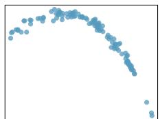
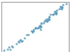
- Linearity. The true relationship between the two variables follows a linear trend. We check whether this is reasonable by examining whether the data follow a linear trend. If there is a nonlinear trend (e.g. left panel of Figure 8.26), an advanced regression method from another book or later course should be applied.
- Nearly normal residuals. For each \(x\)-value, the residuals should be nearly normal. When this assumption is found to be unreasonable, it is usually because of outliers or concerns about influential points. An example that suggests non-normal residuals is shown in the second panel of Figure 8.26. If the sample size \(n \ge 30\), then this assumption is not necessary.
- Constant variability. The variability of points around the true least squares line is constant for all values of \(x\). An example of non-constant variability is shown in the third panel of Figure 8.26.
- Independent. The observations are independent of one another. The observations can be considered independent when they are collected from a random sample or randomized experiment. Be careful of data collected sequentially in what is called a time series. An example of data collected in such a fashion is shown in the fourth panel of Figure 8.26.
We see in Figure 8.26 that patterns in the residual plots suggest that the assumptions for regression inference are not met in those four examples. In fact, identifying nonlinear trends in the data, outliers, and non-constant variability in the residuals is often easier to detect in a residual plot than in a scatterplot.
We note that the second assumption regarding nearly normal residuals is particularly difficult to assess when the sample size is small. We can make a graph, such as a histogram, of the residuals, but we cannot expect a small data set to be nearly normal. All we can do is look for excessive skew or outliers. Outliers and influential points in the data can be seen from the residual plot as well as from a histogram of the residuals.
Conditions for Inference on the Slope of a Regression Line
1. The data is collected from a random sample or randomized experiment.
2. The residual plot appears as a random cloud of points and does not have any patterns or significant outliers that would suggest that the linearity, nearly normal residuals, constant variability, or independence assumptions are unreasonable.
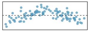
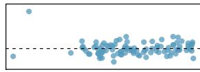
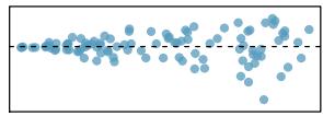
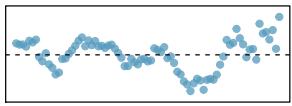
Figure 8.26: Four examples showing when the inference methods in this chapter are insufficient to apply to the data. In the left panel, a straight line does not fit the data. In the second panel, there are outliers: two points on the left are relatively distant from the rest of the data, and one of these points is very far away from the line. In the third panel, the variability of the data around the line increases with larger values of \(x\). In the last panel, a time series data set is shown, where successive observations are highly correlated.
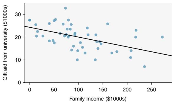
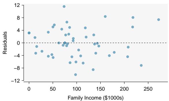
Figure 8.27: Left: Scatterplot of gift aid versus family income for 50 freshmen at Elmhurst College. Right: Residual plot for the model shown in left panel.
Why so many conditions just to test a slope? Because every one of them corresponds to a way the \(t\)-distribution can lie to you. Violating linearity means the regression line itself is the wrong model. Violating constant variability means the standard error is wrong. Violating independence means the whole sampling-distribution story breaks down. The residual plot is your single best diagnostic — one picture, four conditions.
A residual plot is essentially a scatterplot with the linear trend subtracted out. If the line genuinely captures the relationship, what's left over should look like random static. Any pattern you can see in the residuals is a pattern the line failed to capture.
Source: Main Text
You fit a regression line to 40 observations and your residual plot shows the residuals fanning out — small near the left side of the plot and much larger near the right side. Which regression condition is violated, and what does this imply about using the \(t\)-procedures for the slope?
Solution
A fan-shaped residual plot violates the constant variability condition. The typical size of the residuals is not the same for all \(x\)-values, so the standard error for the slope reported by the software will not be trustworthy. The \(t\)-interval and \(t\)-test for the slope should not be applied directly to this data set. A transformation of the variables (like taking a log of \(y\)) or a more advanced regression method would be needed before inference is appropriate.
8.4.3 Constructing a Confidence Interval for the Slope of a Regression Line
We would like to construct a confidence interval for the slope of the regression line for predicting gift aid based on family income for all freshmen at Elmhurst College.
Do conditions seem to be satisfied? We recall that the 50 freshmen in the sample were randomly chosen, so the observations are independent. Next, we need to look carefully at the scatterplot and the residual plot.
Always Check Conditions
Do not blindly apply formulas or rely on regression output; always first look at a scatterplot or a residual plot. If conditions for fitting the regression line are not met, the methods presented here should not be applied.
The scatterplot seems to show a linear trend, which matches the fact that there is no curved trend apparent in the residual plot. Also, the standard deviation of the residuals is mostly constant for different \(x\) values and there are no outliers or influential points. There are no patterns in the residual plot that would suggest that a linear model is not appropriate, so the conditions are reasonably met. We are now ready to calculate the 95% confidence interval.
| Estimate | Std. Error | t value | Pr(>|t|) | |
| (Intercept) | 24.3193 | 1.2915 | 18.83 | 0.0000 |
| family_income | -0.0431 | 0.0108 | -3.98 | 0.0002 |
Figure 8.28: Summary of least squares fit for the Elmhurst College data, where we are predicting gift aid by the university based on the family income of students.
Source: Main Text
Construct a 95% confidence interval for the slope of the regression line for predicting gift aid from family income at Elmhurst College.
Solution
As usual, the confidence interval will take the form:
$$ \text{point estimate} \;\pm\; \text{critical value} \times SE\ \text{of estimate} $$The point estimate for the slope of the population regression line is the slope of the sample regression line: \(-0.0431\). The standard error of the slope can be read from the table as \(0.0108\). Note that we do not need to divide \(0.0108\) by \(\sqrt{n}\) or do any further calculations on \(0.0108\); \(0.0108\) is the \(SE\) of the slope. Note that the value of \(t\) given in the table refers to the test statistic, not the critical value \(t^{\star}\).
To find \(t^{\star}\), we use a \(t\)-table. Here \(n = 50\), so \(df = 50 - 2 = 48\). Using a \(t\)-table, we round down to row \(df = 40\) and estimate the critical value \(t^{\star} = 2.021\) for a 95% confidence level. The confidence interval is calculated as:
$$ -0{.}0431 \pm 2{.}021 \times 0{.}0108 = (-0{.}065,\ -0{.}021) $$Note: \(t^{\star}\) using exactly 48 degrees of freedom is equal to \(2.01\) and gives the same interval of \((-0.065, -0.021)\).
Source: Main Text
Interpret the confidence interval in context. What can we conclude?
Solution
We are 95% confident that the slope of the population regression line — the true average change in gift aid for each additional \$1,000 in family income — is between \(-\$0.065\) thousand dollars and \(-\$0.021\) thousand dollars. That is, we are 95% confident that, on average, when family income is \$1,000 higher, gift aid is between \$21 and \$65 lower.
Because the entire interval is negative, we have evidence that the slope of the population regression line is less than \(0\). In other words, we have evidence that there is a significant negative linear relationship between gift aid and family income.
Constructing a Confidence Interval for the Slope of a Regression Line
To carry out a complete confidence interval procedure to estimate the slope of the population regression line \(\beta\):
Identify: Identify the parameter and the confidence level, C%.
The parameter will be a slope of the population regression line — e.g. the slope of the population regression line relating air quality index to average rainfall per year for each city in the United States.
Choose: Choose the correct interval procedure and identify it by name.
To estimate the slope of a regression model we use a \(t\)-interval for the slope.
Check: Check conditions for using a \(t\)-interval for the slope.
- Independence: Data should come from a random sample or randomized experiment. If sampling without replacement, check that the sample size is less than 10% of the population size.
- Linearity: Check that the scatterplot does not show a curved trend and that the residual plot shows no ∪-shape pattern.
- Constant variability: Use the residual plot to check that the standard deviation of the residuals is constant across all \(x\)-values.
- Normality: The population of residuals is nearly normal or the sample size is \(\ge 30\). If the sample size is less than 30 check for strong skew or outliers in the sample residuals. If neither is found, then the condition that the population of residuals is nearly normal is considered reasonable.
Calculate: Calculate the confidence interval and record it in interval form.
$$ \text{point estimate} \;\pm\; t^{\star} \times SE\ \text{of estimate}, \quad df = n - 2 $$- point estimate: the slope \(b\) of the sample regression line
- \(SE\) of estimate: \(SE\) of slope (find using computer output)
- \(t^{\star}\): use a \(t\)-distribution with \(df = n - 2\) and confidence level C%
Conclude: Interpret the interval and, if applicable, draw a conclusion in context.
We are C% confident that the true slope of the regression line — the average change in \(y\) for each unit increase in \(x\) — is between ___ and ___. If applicable, draw a conclusion based on whether the interval is entirely above, is entirely below, or contains the value \(0\).
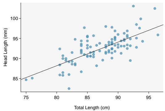
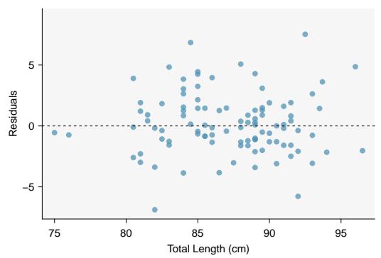
Figure 8.29: Left: Scatterplot of head length versus total length for 104 brushtail possums. Right: Residual plot for the model shown in left panel.
Source: Main Text
The regression summary below shows statistical software output from fitting the least squares regression line for predicting head length from total length for 104 brushtail possums. The scatterplot and residual plot are shown above.
| Predictor | Coef | SE Coef | T | P |
| Constant | 42.70979 | 5.17281 | 8.257 | 5.66e-13 |
| total_length | 0.57290 | 0.05933 | 9.657 | 4.68e-16 |
| S = 2.595 | R-Sq = 47.76% | R-Sq(adj) = 47.25% | ||
Construct a 95% confidence interval for the slope of the regression line. Is there convincing evidence that there is a positive, linear relationship between head length and total length?
Solution
Identify: The parameter of interest is the slope of the population regression line for predicting head length from body length. We want to estimate this at the 95% confidence level.
Choose: Because the parameter to be estimated is the slope of a regression line, we will use the \(t\)-interval for the slope.
Check: These data come from a random sample. The residual plot shows no pattern, so a linear model seems reasonable. The residual plot also shows that the residuals have constant standard deviation. Finally, \(n = 104 \ge 30\) so we do not have to check for skew in the residuals. All four conditions are met.
Calculate: We will calculate the interval: \(\text{point estimate} \pm t^{\star} \times SE\ \text{of estimate}\).
We read the slope of the sample regression line and the corresponding \(SE\) from the table. The point estimate is \(b = 0.57290\). The \(SE\) of the slope is \(0.05933\), which can be found next to the slope of \(0.57290\). The degrees of freedom is \(df = n - 2 = 104 - 2 = 102\). As before, we find the critical value \(t^{\star}\) using a \(t\)-table (the \(t^{\star}\) value is not the same as the \(T\)-statistic for the hypothesis test). Using the \(t\)-table at row \(df = 100\) (round down since 102 is not on the table) and confidence level 95%, we get \(t^{\star} = 1.984\).
So the 95% confidence interval is given by:
$$ 0{.}57290 \pm 1{.}984 \times 0{.}05933 $$ $$ (0{.}456,\ 0{.}691) $$Conclude: We are 95% confident that the slope of the population regression line is between \(0.456\) and \(0.691\). That is, we are 95% confident that the true average increase in head length for each additional cm in total length is between \(0.456\) mm and \(0.691\) mm. Because the interval is entirely above \(0\), we do have evidence of a positive linear association between head length and body length for brushtail possums.
Source: Main Text
Figure 8.21 shows statistical software output from fitting the least squares regression line shown in Figure 8.15. Use this output to formally evaluate the following hypotheses.
\(H_0\): The true coefficient for family income is zero.
\(H_A\): The true coefficient for family income is not zero.
Figure 8.21: Summary of least squares fit for the Elmhurst College data, where we are predicting the gift aid by the university based on the family income of students.
| Estimate | Std. Error | t value | Pr(>|t|) | |
| (Intercept) | 24319.3 | 1291.5 | 18.83 | <0.0001 |
| family_income | -0.0431 | 0.0108 | -3.98 | 0.0002 |
| df = 48 |
Solution
From the table, the point estimate is \(b = -0.0431\) with \(SE = 0.0108\) on \(df = 48\). The reported test statistic is
$$ T = \frac{-0{.}0431 - 0}{0{.}0108} = -3{.}98, $$and the two-sided p-value is \(0.0002\). Since the p-value is far below any standard significance level (e.g. \(\alpha = 0.05\)), we reject \(H_0\). The data provide convincing evidence that the true coefficient for family income is not zero — i.e. there is a real linear relationship between family income and gift aid at Elmhurst College.


Every confidence interval for a slope is also a hypothesis test in disguise. If \(0\) is inside the interval, you cannot rule out "no linear relationship." If \(0\) is outside, you can. For the Elmhurst data the interval is \((-0.065, -0.021)\) — entirely negative — which matches the test's conclusion that \(\beta \ne 0\).
Source: Main Text
A regression of a child's reading score on time spent reading at home (hours/week) for \(n = 25\) students gives \(b = 1.6\) with \(SE = 0.55\). Assume the four conditions for slope inference are met.
(a) What is the critical value \(t^{\star}\) for a 95% confidence interval, using \(df = n - 2\)? (Use \(df = 20\) from the table.) (b) Compute the 95% confidence interval for \(\beta\). (c) Does the interval contain \(0\)? What does that tell you?
Solution
(a) \(df = 25 - 2 = 23\). Rounding down to \(df = 20\) in the \(t\)-table, \(t^{\star} \approx 2.086\).
(b) CI: \(1.6 \pm 2.086 \times 0.55 = 1.6 \pm 1.147 = (0.453,\ 2.747)\).
(c) The interval is entirely above \(0\), so we have evidence of a positive linear relationship between time spent reading at home and reading score. Each additional hour per week is associated with an increase of roughly \(0.45\) to \(2.75\) points on the reading score, on average.
The critical value \(t^{\star}\) and the test statistic \(T\) are easy to confuse because they're both on the \(t\)-distribution and both look like "t-something." Keep them distinct: \(t^{\star}\) is a table lookup determined only by \(df\) and the confidence level — it never depends on your data. \(T\) is computed from your data and measures how far the observed slope is from zero in standard-error units. Mixing them up is the single most common slope-inference error.
8.4.4 Midterm Elections and Unemployment
Elections for members of the United States House of Representatives occur every two years, coinciding every four years with the U.S. Presidential election. The set of House elections occurring during the middle of a Presidential term are called midterm elections. In America's two-party system, one political theory suggests the higher the unemployment rate, the worse the President's party will do in the midterm elections.
To assess the validity of this claim, we can compile historical data and look for a connection. We consider every midterm election from 1898 to 2018, with the exception of those elections during the Great Depression. Figure 8.30 shows these data and the least-squares regression line:
% change in House seats for President's party
$$ = -7{.}36 - 0{.}89 \times (\text{unemployment rate}) $$We consider the percent change in the number of seats of the President's party (e.g. percent change in the number of seats for Republicans in 2018) against the unemployment rate.
Examining the data, there are no clear deviations from linearity, the constant variance condition, or the normality of residuals. While the data are collected sequentially, a separate analysis was used to check for any apparent correlation between successive observations; no such correlation was found.
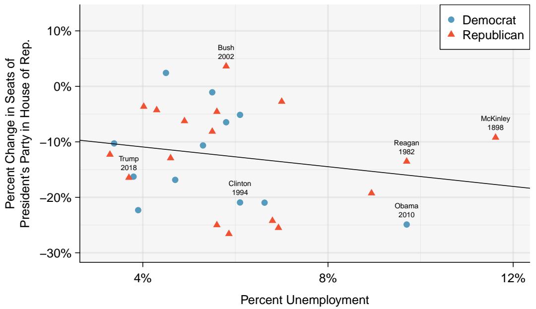
Figure 8.30: The percent change in House seats for the President's party in each election from 1898 to 2018 plotted against the unemployment rate. The two points for the Great Depression have been removed, and a least squares regression line has been fit to the data.

Source: Main Text
The data for the Great Depression (1934 and 1938) were removed because the unemployment rate was 21% and 18%, respectively. Do you agree that they should be removed for this investigation? Why or why not?
Solution
There is a reasonable case for removing these two observations. Unemployment rates of 21% and 18% are extreme outliers compared to every other midterm election in the data set — they are far outside the typical range of unemployment rates during the last century. As influential points, they could pull the regression line dramatically and make it less representative of the typical midterm election relationship we are trying to describe.
That said, removing outliers is never neutral. A reader of the analysis should be told that these points were dropped and given the reasoning. A responsible write-up reports the results both with and without them, so the audience can judge how sensitive the conclusion is to the Great Depression observations.
There is a negative slope in the line shown in Figure 8.30. However, this slope (and the \(y\)-intercept) are only estimates of the parameter values. We might wonder, is this convincing evidence that the "true" linear model has a negative slope? That is, do the data provide strong evidence that the political theory is accurate? We can frame this investigation as a statistical hypothesis test:
\(H_0\): \(\beta = 0\). The true linear model has slope zero.
\(H_A\): \(\beta < 0\). The true linear model has a slope less than zero. The higher the unemployment, the greater the loss for the President's party in the House of Representatives.
We would reject \(H_0\) in favor of \(H_A\) if the data provide strong evidence that the slope of the population regression line is less than zero. To assess the hypotheses, we identify a standard error for the estimate, compute an appropriate test statistic, and identify the p-value.
Testing for the Slope Using a Cutoff of 0.05
What does it mean to say that the slope of the population regression line is significantly greater than \(0\)? And why do we tend to use a cutoff of \(\alpha = 0.05\)? See the 5-minute interactive task at www.openintro.org/why05 for an explanation.
Statistical significance is not the same as practical significance. A slope of \(-0.89\) means roughly \(0.89\) percentage points of seats lost for every 1 percentage point higher unemployment — that is a real political story. But whether the data prove that story is a separate question, and it's the one the hypothesis test answers.
When the data refuse to reject \(H_0\), it doesn't mean "there is no relationship." It means "with this sample size and this amount of noise, we can't rule out zero." The absence of evidence is not evidence of absence — it is a call for more data or a different study.
Source: Main Text
Using the midterm-election regression (slope \(b = -0.8897\), \(SE = 0.8350\), \(n = 27\)), carry out a one-sided test of \(H_0: \beta = 0\) vs. \(H_A: \beta < 0\) at \(\alpha = 0.05\).
(a) What is the test statistic \(T\)? (b) What are the degrees of freedom? (c) Given that the two-sided p-value from the output is \(0.2961\), what is the one-sided p-value? (d) State the conclusion in context.
Solution
(a) \(T = \dfrac{-0{.}8897 - 0}{0{.}8350} = -1{.}07\).
(b) \(df = n - 2 = 27 - 2 = 25\).
(c) The one-sided p-value is half the two-sided value: \(0.2961 / 2 \approx 0.148\). This halving is valid only because our observed slope (\(-0.8897\)) is in the direction of \(H_A\) (negative).
(d) The one-sided p-value \(\approx 0.148\) is much larger than \(\alpha = 0.05\), so we fail to reject \(H_0\). The data do not provide convincing evidence that higher unemployment is associated with a larger loss of House seats for the President's party in midterm elections.
8.4.5 Understanding Regression Output from Software
The residual plot shown in Figure 8.31 shows no pattern that would indicate that a linear model is inappropriate. Therefore we can carry out a test on the population slope using the sample slope as our point estimate. Just as for other point estimates we have seen before, we can compute a standard error and test statistic for \(b\). The test statistic \(T\) follows a \(t\)-distribution with \(n - 2\) degrees of freedom.
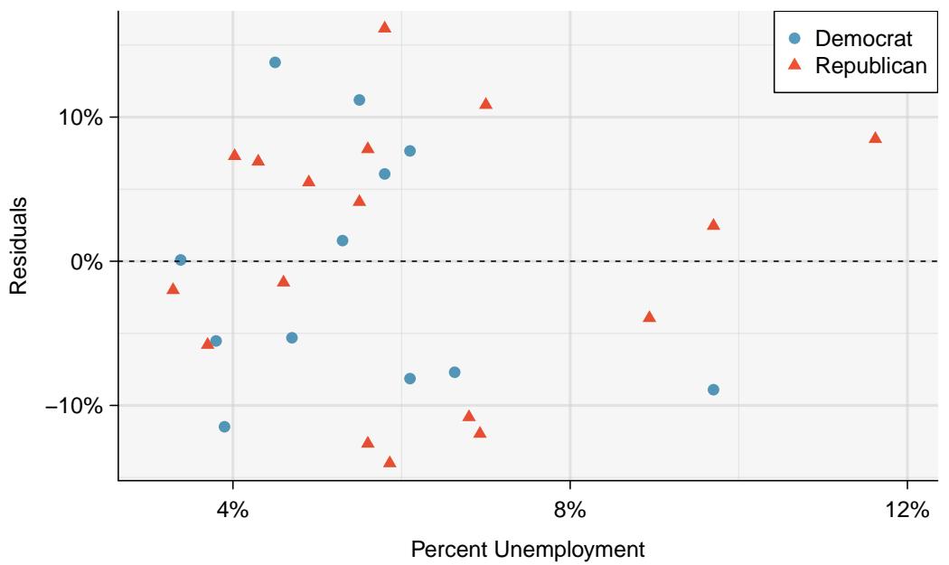
Figure 8.31: The residual plot shows no pattern that would indicate that a linear model is inappropriate.
Hypothesis Tests on the Slope of the Regression Line
Use a \(t\)-test with \(n - 2\) degrees of freedom when performing a hypothesis test on the slope of a regression line.
We will rely on statistical software to compute the standard error and leave the explanation of how this standard error is determined to a second or third statistics course. Figure 8.32 shows software output for the least squares regression line in Figure 8.30. The row labeled unemp represents the information for the slope, which is the coefficient of the unemployment variable.
Figure 8.32: Least squares regression summary for the percent change in seats of President's party in House of Representatives based on percent unemployment.
| Estimate | Std. Error | t value | Pr(>|t|) | |
| (Intercept) | -7.3644 | 5.1553 | -1.43 | 0.1646 |
| unemp | -0.8897 | 0.8350 | -1.07 | 0.2961 |
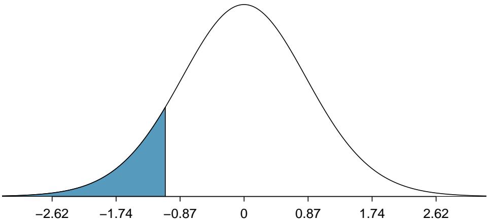
Figure 8.33: The distribution shown here is the sampling distribution for \(b\), if the null hypothesis was true. The shaded tail represents the p-value for the hypothesis test evaluating whether there is convincing evidence that higher unemployment corresponds to a greater loss of House seats for the President's party during a midterm election.
Source: Main Text
What do the first column of numbers in the regression summary represent?
Solution
The entries in the first column represent the least squares estimates for the \(y\)-intercept and slope, \(a\) and \(b\) respectively. Using this information, we could write the equation for the least squares regression line as
$$ \hat{y} = -7{.}3644 - 0{.}8897 x, $$where \(y\) in this case represents the percent change in the number of seats for the President's party, and \(x\) represents the unemployment rate.
We previously used a test statistic \(T\) for hypothesis testing in the context of means. Regression is very similar. Here, the point estimate is \(b = -0.8897\). The \(SE\) of the estimate is \(0.8350\), which is given in the second column next to the estimate of \(b\). This \(SE\) represents the typical error when using the slope of the sample regression line to estimate the slope of the population regression line.
The null value for the slope is \(0\), so we now have everything we need to compute the test statistic. We have:
$$ T = \frac{\text{point estimate} - \text{null value}}{SE\ \text{of estimate}} = \frac{-0{.}8897 - 0}{0{.}8350} = -1{.}07 $$This value corresponds to the \(T\)-score reported in the regression output in the third column along the unemp row.
Source: Main Text
In this example, the sample size \(n = 27\). Identify the degrees of freedom and p-value for the hypothesis test.
Solution
The degrees of freedom are \(df = n - 2 = 27 - 2 = 25\). For a two-sided test, the p-value is the area in the two tails beyond \(\pm T = \pm 1.07\) on a \(t\)-distribution with \(df = 25\), which equals \(0.2961\) as reported in the last column of the table.
Because the p-value is so large, we do not reject the null hypothesis. That is, the data do not provide convincing evidence that a higher unemployment rate is associated with a larger loss for the President's party in the House of Representatives in midterm elections.
Don't Carelessly Use the P-Value from Regression Output
The last column in regression output often lists p-values for one particular hypothesis: a two-sided test where the null value is zero. If your test is one-sided and the point estimate is in the direction of \(H_A\), then you can halve the software's p-value to get the one-tail area. If neither of these scenarios matches your hypothesis test, be cautious about using the software output to obtain the p-value.
Source: Main Text
Use the table in Figure 8.20 to determine the p-value for the hypothesis test.

Solution
The last column of the table gives the p-value for the two-sided hypothesis test for the coefficient of the unemployment rate: \(0.2961\). That is, the data do not provide convincing evidence that a higher unemployment rate has any correspondence with smaller or larger losses for the President's party in the House of Representatives in midterm elections.
Hypothesis Test for the Slope of a Regression Line
To carry out a complete hypothesis test for the claim that there is no linear relationship between two numerical variables, i.e. that \(\beta = 0\):
Identify: Identify the hypotheses and the significance level, \(\alpha\).
$$ H_0: \beta = 0 $$ $$ H_A: \beta \ne 0, \quad H_A: \beta > 0, \quad \text{or} \quad H_A: \beta < 0 $$Choose: Choose the correct test procedure and identify it by name.
To test hypotheses about the slope of a regression model we use a \(t\)-test for the slope.
Check: Check conditions for using a \(t\)-test for the slope (the same four conditions as for the interval).
Calculate: Calculate the \(t\)-statistic, \(df\), and p-value.
$$ T = \frac{\text{point estimate} - \text{null value}}{SE\ \text{of estimate}}, \quad df = n - 2 $$- point estimate: the slope \(b\) of the sample regression line
- \(SE\) of estimate: \(SE\) of slope (find using computer output)
- null value: \(0\)
- p-value: based on the \(t\)-statistic, the \(df\), and the direction of \(H_A\)
Conclude: Compare the p-value to \(\alpha\), and draw a conclusion in context.
- If the p-value \(< \alpha\), reject \(H_0\); there is sufficient evidence that [\(H_A\) in context].
- If the p-value \(> \alpha\), do not reject \(H_0\); there is not sufficient evidence that [\(H_A\) in context].
Source: Main Text
The regression summary below shows statistical software output from fitting the least squares regression line for predicting gift aid based on family income for 50 randomly selected freshman students at Elmhurst College. The scatterplot and residual plot were shown in Figure 8.27.
| Predictor | Coef | SE Coef | T | P |
| Constant | 24.31933 | 1.29145 | 18.831 | < 2e-16 |
| family_income | -0.04307 | 0.01081 | -3.985 | 0.000229 |
Do these data provide convincing evidence that there is a negative, linear relationship between family income and gift aid? Carry out a complete hypothesis test at the 0.05 significance level. Use the five step framework to organize your work.
Solution
Identify: We will test the following hypotheses at the \(\alpha = 0.05\) significance level.
\(H_0\): \(\beta = 0\). There is no linear relationship.
\(H_A\): \(\beta < 0\). There is a negative linear relationship.
Here, \(\beta\) is the slope of the population regression line for predicting gift aid from family income at Elmhurst College.
Choose: Because the hypotheses are about the slope of a regression line, we choose the \(t\)-test for a slope.
Check: The data come from a random sample of less than 10% of the total population of freshman students at Elmhurst College. The lack of any pattern in the residual plot indicates that a linear model is reasonable. Also, the residual plot shows that the residuals have constant variance. Finally, \(n = 50 \ge 30\) so we do not have to worry too much about any skew in the residuals. All four conditions are met.
Calculate: We will calculate the \(t\)-statistic, degrees of freedom, and the p-value.
We read the slope of the sample regression line and the corresponding \(SE\) from the table.
- The point estimate is: \(b = -0.04307\). - The \(SE\) of the slope is: \(SE = 0.01081\).
$$ T = \frac{-0{.}04307 - 0}{0{.}01081} = -3{.}985 $$Because \(H_A\) uses a less-than sign (\(<\)), meaning that it is a lower-tail test, the p-value is the area to the left of \(t = -3.985\) under the \(t\)-distribution with \(50 - 2 = 48\) degrees of freedom.
$$ \text{p-value} = \tfrac{1}{2}(0{.}000229) \approx 0{.}0001 $$Conclude: The p-value of \(0.0001\) is \(< 0.05\), so we reject \(H_0\); there is sufficient evidence that there is a negative linear relationship between family income and gift aid at Elmhurst College.
Source: Main Text
In context, interpret the p-value from the previous example.
Solution
The p-value of roughly \(0.0001\) is the probability of observing a sample slope as extreme as \(b = -0.04307\) — or more extreme in the direction of \(H_A\) — if the true slope of the population regression line really were zero (i.e., if there were no linear relationship between family income and gift aid).
Because this probability is so tiny, the observed slope is very hard to explain by random chance alone. That is why we reject \(H_0\): the data are inconsistent with the "no-relationship" hypothesis, and we instead conclude that higher family income is genuinely associated with lower gift aid at Elmhurst College.
Source: Main Text
In a regression summary, the row for the predictor study_hours shows Estimate \(= 3.2\), Std. Error \(= 0.9\), t value \(= 3.56\), and \(\Pr(>|t|) = 0.0006\). The sample size is \(n = 42\).
(a) What are the hypotheses corresponding to the reported p-value? (b) Explain what the \(t\) value column was computed from. (c) At \(\alpha = 0.01\), what do you conclude about \(\beta\)?
Solution
(a) The reported p-value is two-sided, so \(H_0: \beta = 0\) vs. \(H_A: \beta \ne 0\).
(b) \(t = b / SE = 3.2 / 0.9 \approx 3.56\). It's the standardized distance from the null slope of \(0\), measured in standard errors.
(c) \(p = 0.0006 < 0.01\), so we reject \(H_0\). There is convincing evidence that the true slope of the population regression line is not zero — study_hours has a nonzero linear association with the response variable.
Regression output tables look intimidating but carry only four pieces of information per row: the point estimate, its standard error, the \(t\)-statistic, and the two-sided p-value. That's it. Every statistical-software vendor uses different column labels (Coef, Estimate, Coefficient, b), but the meaning is the same. Once you can read one table you can read them all.
The p-values reported in regression output are always two-sided tests of \(H_0: \beta = 0\). If your research question is one-sided ("does \(x\) increase \(y\)?"), halve the reported p-value — but only if your observed slope is in the direction of \(H_A\). If the observed slope is opposite to \(H_A\), the correct one-sided p-value is actually \(1 - p/2\), which will be close to 1. Mindlessly halving without checking direction is a common mistake.
8.4.6 Technology: the \(t\)-test/Interval for the Slope
We generally rely on regression output from statistical software programs to provide us with the necessary quantities: \(b\) and \(SE\) of \(b\). However we can also find the test statistic, p-value, and confidence interval using Desmos or a handheld calculator.
Get started quickly with the Desmos T-Test/Interval Calculator (available at openintro.org/ahss/desmos).
For instructions on implementing the T-Test/Interval on the TI or Casio, see the Graphing Calculator Guides at openintro.org/ahss.
Inference for Regression
We usually rely on statistical software to identify point estimates, standard errors, test statistics, and p-values in practice. However, be aware that software will not generally check whether the method is appropriate, meaning we must still verify conditions are met.
Software makes slope inference nearly effortless — you feed it two columns and it hands you a full regression table. The price of that convenience is a tendency to skip the residual plot. A significant p-value from a regression that violates linearity or constant variability is worse than no p-value at all, because it feels authoritative. Always look at the picture before you quote the number.
Every entry in the regression table has a familiar analog: Estimate is \(b\), Std. Error is \(SE\), t value is \(b/SE\), and Pr(>|t|) is the two-sided p-value. Once you see the pattern, every new software package becomes readable in seconds.
Source: Main Text
You type a data set of \(n = 30\) paired observations into software and the row for your predictor reads Estimate \(= -0.42\), Std. Error \(= 0.25\), t value \(= -1.68\), \(\Pr(>|t|) = 0.104\).
(a) Verify the reported \(t\) value by hand from the Estimate and Std. Error. (b) What is the two-sided p-value for \(H_0: \beta = 0\)? (c) Build a 95% confidence interval for \(\beta\) using \(t^{\star} \approx 2.048\) (from \(df = 28\)). (d) Does your interval include \(0\)? Is that consistent with the reported p-value at \(\alpha = 0.05\)?
Solution
(a) \(t = -0.42 / 0.25 = -1.68\). Matches the table.
(b) The two-sided p-value is \(0.104\) — read directly from the output.
(c) CI: \(-0.42 \pm 2.048 \times 0.25 = -0.42 \pm 0.512 = (-0.932,\ 0.092)\).
(d) Yes, the interval contains \(0\). This is consistent with the p-value \(0.104 > 0.05\): we fail to reject \(H_0\) at the 5% level, which is exactly what "zero is in the interval" tells us.
8.4.7 Which Inference Procedure to Use for Paired Data?
In Section 7.2.4, we looked at a set of paired data involving the price of textbooks for UCLA courses at the UCLA Bookstore and on Amazon. The left panel of Figure 8.34 shows the difference in price (UCLA Bookstore − Amazon) for each book. Because we have two data points on each textbook, it also makes sense to construct a scatterplot, as seen in the right panel of Figure 8.34.
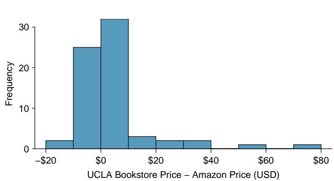
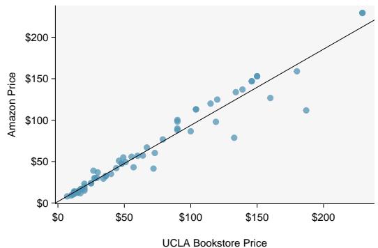
Figure 8.34: Left: histogram of the difference (UCLA Bookstore price − Amazon price) for each book sampled. Right: scatterplot of Amazon Price versus UCLA Bookstore price.
Source: Main Text
What additional information does the scatterplot provide about the price of textbooks at UCLA Bookstore and on Amazon?
Solution
With a scatterplot, we see the relationship between the variables. We can see that when UCLA Bookstore price is larger, Amazon price also tends to be larger. We can consider the strength of the correlation, and we can draw the linear regression equation for predicting Amazon price from UCLA Bookstore price.
Source: Main Text
Which test should we do if we want to check whether:
1. prices for textbooks for UCLA courses are higher at the UCLA Bookstore than on Amazon; 2. there is a significant, positive linear relationship between UCLA Bookstore price and Amazon price?
Solution
In the first case, we are interested in whether the differences (UCLA Bookstore − Amazon) for all UCLA textbooks are, on average, greater than \(0\), so we would do a one-sample \(t\)-test for a mean of differences. In the second case, we are interested in whether the slope of the regression line for predicting Amazon price from UCLA Bookstore price is significantly greater than \(0\), so we would do a \(t\)-test for the slope of a regression line.
Likewise, a one-sample \(t\)-interval for a mean of differences would provide an interval of reasonable values for the mean of differences in textbook price between UCLA Bookstore and Amazon (for all UCLA textbooks), while a \(t\)-interval for the slope would provide an interval of reasonable values for the slope of the regression line for predicting Amazon price from UCLA Bookstore price (for all UCLA textbooks).
Inference for Paired Data
A one-sample \(t\)-interval or \(t\)-test for a mean of differences only makes sense when we are asking whether, on average, one variable is greater than, less than, or different from another (think histogram of the differences). A \(t\)-interval or \(t\)-test for the slope of a regression line makes sense when we are interested in the linear relationship between them (think scatterplot).
Source: Main Text
Previously, we looked at the relationship between body length and head length for brushtail possums. We also looked at the relationship between gift aid and family income for freshmen at Elmhurst College. Could we do a one-sample \(t\)-test in either of these scenarios?
Solution
We have to ask ourselves: does it make sense to ask whether, on average, body length is greater than head length? Similarly, does it make sense to ask whether, on average, gift aid is greater than family income? These don't seem to be meaningful research questions; a one-sample \(t\)-test for a mean of differences would not be useful here.
Source: Main Text
A teacher gives her class a pretest and a posttest. Does this result in paired data? If so, which hypothesis test should she use?
Solution
Yes, this is paired data — each student contributes two observations (pretest score, posttest score), and the pairing is meaningful because the two scores come from the same individual.
The natural question is "did scores change, on average, between pretest and posttest?" That's a question about the mean of the differences (posttest − pretest), so she should use a one-sample \(t\)-test for a mean of differences. A \(t\)-test for a slope would only be appropriate if she wanted to model posttest score as a linear function of pretest score — a different question.
Source: Main Text
For each research question, state whether the appropriate procedure is a one-sample \(t\)-test for a mean of differences or a \(t\)-test for the slope of a regression line.
(a) Among married couples in a city, is the husband's age, on average, greater than the wife's age? (b) Among the same couples, is there a positive linear relationship between husband's age and wife's age? (c) In a study of twins, is the first-born twin's birth weight typically different from the second-born's? (d) In the same study, does a heavier first-born twin tend to predict a heavier second-born twin?
Solution
(a) One-sample \(t\)-test for a mean of differences. The question is about the typical difference (husband − wife) being different from \(0\).
(b) \(t\)-test for the slope. The question is whether the two variables have a linear association.
(c) One-sample \(t\)-test for a mean of differences. The question asks about the average difference in birth weight between first- and second-born twins.
(d) \(t\)-test for the slope. The question is about a linear relationship between the two weights, not the average difference.
"Paired data" by itself doesn't dictate which test to use — what matters is the question you're asking. A histogram-shaped question ("is \(A\) on average bigger than \(B\)?") is a paired \(t\)-test. A scatterplot-shaped question ("when \(A\) goes up, does \(B\) go up too?") is a slope test. The same two columns of numbers can appropriately feed either test; the research question chooses.
The paired \(t\)-test and the slope test are not substitutes — they answer orthogonal questions. It's perfectly reasonable for a dataset to show a significant paired difference but a non-significant slope, or vice versa. If both tests feel relevant, you probably need both: report the mean difference and the correlation.
Section Summary
In Chapter 6, we used a \(\chi^2\) test for independence to test for association between two categorical variables. In this section, we test for association/correlation between two numerical variables.
- We use the slope \(b\) as a point estimate for the slope \(\beta\) of the population regression line. The slope of the population regression line is the true increase/decrease in \(y\) for each unit increase in \(x\). If the slope of the population regression line is \(0\), there is no linear relationship between the two variables.
- Under certain assumptions, the sampling distribution for \(b\) is normal and the distribution of the standardized test statistic using the standard error of the slope follows a \(t\)-distribution with \(n - 2\) degrees of freedom.
- When there is \((x, y)\) data and the parameter of interest is the slope of the population regression line:
- Estimate \(\beta\) at the C% confidence level using a \(t\)-interval for the slope.
- Test \(H_0: \beta = 0\) at the \(\alpha\) significance level using a \(t\)-test for the slope.
- The conditions for the \(t\)-interval and \(t\)-test for the slope of a regression line are the same:
- 1. Independence: Data come from a random sample or randomized experiment. If sampling without replacement, check that the sample size is less than 10% of the population size.
- 2. Linearity: Check that the scatterplot does not show a curved trend and that the residual plot shows no ∪-shape pattern.
- 3. Constant variability: Use the residual plot to check that the standard deviation of the residuals is constant across all \(x\)-values.
- 4. Normality: The population of residuals is nearly normal or the sample size is \(\ge 30\). If the sample size is less than 30, check for strong skew or outliers in the sample residuals.
- The confidence interval and test statistic are calculated as follows:
- The confidence interval for the slope of the population regression line estimates the true average increase in the \(y\)-variable for each unit increase in the \(x\)-variable.
- The \(t\)-test for the slope and the one-sample \(t\)-test for a mean of differences both involve paired, numerical data. However, the \(t\)-test for the slope asks if the two variables have a linear relationship — specifically, if the slope of the population regression line is different from \(0\). The one-sample \(t\)-test for a mean of differences asks if the two variables are, on average, different — specifically, if the mean of the population differences is not equal to \(0\).
Problem Set — Section 8.4
Source: Main Text
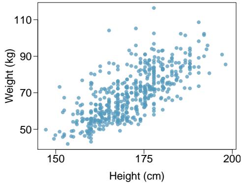
Problem 1: Body measurements, Part IV. The scatterplot and least squares summary below show the relationship between weight measured in kilograms and height measured in centimeters of 507 physically active individuals.
| Estimate | Std. Error | t value | Pr(>|t|) | |
| (Intercept) | -105.0113 | 7.5394 | -13.93 | 0.0000 |
| height | 1.0176 | 0.0440 | 23.13 | 0.0000 |
(a) Describe the relationship between height and weight.
(b) Write the equation of the regression line. Interpret the slope and intercept in context.
(c) Do the data provide strong evidence that an increase in height is associated with an increase in weight? State the null and alternative hypotheses, report the p-value, and state your conclusion.
(d) The correlation coefficient for height and weight is \(0.72\). Calculate \(R^2\) and interpret it in context.
Problem 8.33 Solution
Step 1 — Describe the relationship (a): The scatterplot shows a positive, roughly linear association between height and weight for physically active individuals: taller people tend to weigh more. The spread is moderate and reasonably constant across the range of heights, with no obvious outliers.
Step 2 — Write the regression equation (b):
Using the Estimate column:
$$\widehat{\text{weight}} = -105.0113 + 1.0176 \times \text{height}.$$
Slope interpretation: For each additional 1 cm in height, we predict an increase of about \(1.018\) kg in weight, on average. Intercept interpretation: The intercept is the predicted weight when height is \(0\) cm — not meaningful here, since nobody is 0 cm tall.
Step 3 — Hypothesis test for the slope (c):
Hypotheses: \(H_0: \beta = 0\) vs. \(H_A: \beta \neq 0\). The regression output reports \(T = 23.13\) and p-value \(0.0000\) for the height row. Since \(p < 0.05\), we reject \(H_0\). The data provide very strong evidence that increases in height are associated with increases in weight.
Step 4 — Compute \(R^2\) (d): $$R^2 = r^2 = (0.72)^2 = 0.5184.$$ About 52% of the variability in weight among these physically active individuals is explained by a linear model using height as the predictor.
Answer: (a) Positive, roughly linear. (b) \(\widehat{\text{weight}} = -105.01 + 1.018 \times \text{height}\). (c) Reject \(H_0\); strong evidence of a positive linear association (\(p \approx 0\)). (d) \(R^2 \approx 0.52\).
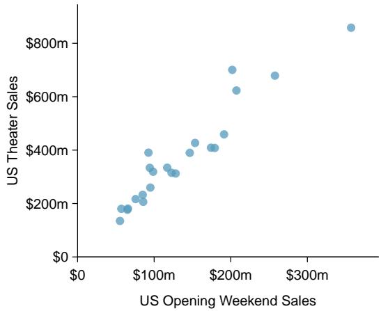
Problem 2: MCU, predict US theater sales. The Marvel Comic Universe movies were an international movie sensation, containing 23 movies at the time of this writing. Here we consider a model predicting an MCU film's gross theater sales in the US based on the first weekend sales performance in the US. The data are presented below in both a scatterplot and the model in a regression table. Scientific notation is used below — e.g. 42.5e6 corresponds to \(42.5 \times 10^6\).
| Estimate | Std. Error | t value | Pr(>|t|) | |
| (Intercept) | 42.5e6 | 26.6e6 | 1.60 | 0.1251 |
| opening_wednesday_us | 2.4361 | 0.1739 | 14.01 | 0.0000 |
(a) Describe the relationship between gross theater sales in the US and first weekend sales in the US.
(b) Write the equation of the regression line. Interpret the slope and intercept in context.
(c) Do the data provide strong evidence that higher opening weekend sales are associated with higher gross theater sales? State the null and alternative hypotheses, report the p-value, and state your conclusion.
(d) The correlation coefficient for gross sales and first weekend sales is \(0.950\). Calculate \(R^2\) and interpret it in context.
(e) Suppose we consider a set of all films ever released. Do you think the relationship between opening weekend sales and total sales would be as strong as what we see with the MCU films?
Problem 8.34 Solution
Step 1 — Describe the relationship (a): Gross US theater sales increase strongly and approximately linearly with opening-weekend US sales: higher opening weekends correspond to higher totals, with little deviation from a straight line.
Step 2 — Regression equation (b): $$\widehat{\text{gross}} = 42.5 \times 10^{6} + 2.4361 \times \text{opening\_wed\_us}.$$ Slope: Each additional \$1 of opening-Wednesday sales is associated with an additional \$2.44 in total US gross, on average. Intercept: The predicted gross for a hypothetical film with \$0 opening-Wednesday sales is about \$42.5 million — extrapolation outside the observed range, so interpret with caution.
Step 3 — Hypothesis test (c): \(H_0: \beta = 0\) vs. \(H_A: \beta \neq 0\). The table shows \(T = 14.01\) and p-value \(0.0000\). Since \(p < 0.05\), we reject \(H_0\). Higher opening weekend sales are strongly associated with higher gross sales.
Step 4 — Compute \(R^2\) (d): $$R^2 = (0.950)^2 = 0.9025.$$ About 90% of the variability in MCU gross sales is explained by opening-weekend sales.
Step 5 — Generalize (e): Probably not. MCU films are a highly curated, heavily marketed franchise with similar audiences. In a set of all films, budgets, genres, and distribution vary far more, so opening weekends would still correlate with total sales but almost certainly with a much lower \(R^2\) and more scatter.
Answer: (a) Strong positive linear. (b) \(\hat{y} = 42.5\text{M} + 2.44 x\). (c) Reject \(H_0\); very strong positive association. (d) \(R^2 \approx 0.90\). (e) Expect a weaker relationship for all films.
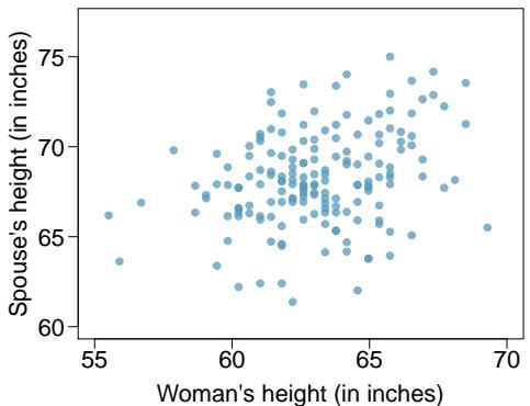
Problem 3: Spouses, Part II. The scatterplot below summarizes women's heights and their spouses' heights for a random sample of 170 married women in Britain, where both partners' ages are below 65 years. Summary output of the least squares fit for predicting spouse's height from the woman's height is also provided in the table.
| Estimate | Std. Error | t value | Pr(>|t|) | |
| (Intercept) | 43.5755 | 4.6842 | 9.30 | 0.0000 |
| height_spouse | 0.2863 | 0.0686 | 4.17 | 0.0000 |
(a) Is there strong evidence in this sample that taller women have taller spouses? State the hypotheses and include any information used to conduct the test.
(b) Write the equation of the regression line for predicting the height of a woman's spouse based on the woman's height.
(c) Interpret the slope and intercept in the context of the application.
(d) Given that \(R^2 = 0.09\), what is the correlation of heights in this data set?
(e) You meet a married woman from Britain who is 5'9" (69 inches). What would you predict her spouse's height to be? How reliable is this prediction?
(f) You meet another married woman from Britain who is 6'7" (79 inches). Would it be wise to use the same linear model to predict her spouse's height? Why or why not?
Problem 8.35 Solution
Step 1 — State and evaluate the hypotheses (a): \(H_0: \beta = 0\) vs. \(H_A: \beta \neq 0\). Using the regression table: slope \(b = 0.2863\), \(SE = 0.0686\), \(T = 4.17\), p-value \(0.0000\). With \(n = 170\), \(df = 168\). Since \(p < 0.05\), we reject \(H_0\) and conclude there is strong evidence that taller women have taller spouses.
Step 2 — Regression equation (b): $$\widehat{\text{spouse\_height}} = 43.5755 + 0.2863 \times \text{woman\_height}.$$
Step 3 — Slope and intercept in context (c): Slope: For each additional inch in a woman's height, the spouse's predicted height increases by about \(0.29\) inches, on average. Intercept: A woman of height 0 inches is predicted to have a spouse of height \(43.6\) inches — not meaningful; it is only a mathematical baseline.
Step 4 — Correlation from \(R^2\) (d): $$r = \pm\sqrt{0.09} = \pm 0.30.$$ The slope is positive, so \(r = +0.30\).
Step 5 — Prediction for 69 inches (e): $$\widehat{\text{spouse}} = 43.5755 + 0.2863 \times 69 = 43.5755 + 19.7547 \approx 63.33 \text{ in.}$$ Because \(R^2 = 0.09\) is small, individual predictions are unreliable — height explains only \(\approx 9\%\) of spouse-height variation.
Step 6 — Prediction for 79 inches (f): No — \(79\) inches (6'7") is far above the sampled range. Using the line there is extrapolation, and the linear relationship may not hold at the extremes.
Answer: (a) Reject \(H_0\); strong evidence. (b) \(\hat{y} = 43.58 + 0.286 x\). (c) See step 3. (d) \(r \approx 0.30\). (e) \(\approx 63.3\) in; weak prediction. (f) No — extrapolation.
Problem 4: Urban homeowners, Part II. Exercise 8.29 gives a scatterplot displaying the relationship between the percent of families that own their home and the percent of the population living in urban areas. Below is a similar scatterplot, excluding District of Columbia, as well as the residuals plot. There were 51 cases.
(a) For these data, \(R^2 = 0.28\). What is the correlation? How can you tell if it is positive or negative?
(b) Examine the residual plot. What do you observe? Is a simple least squares fit appropriate for these data?
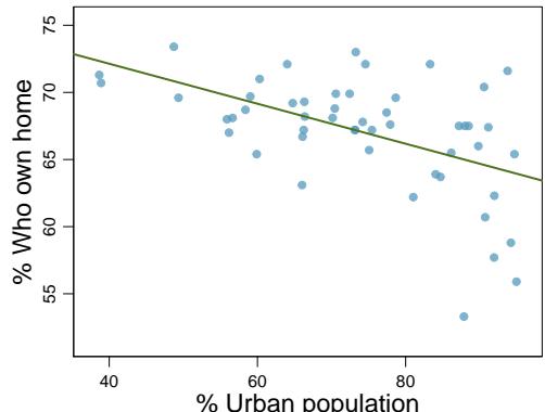
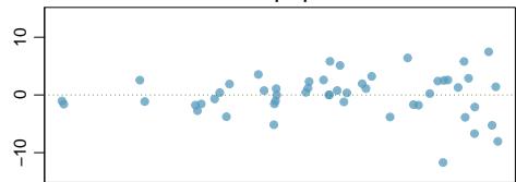
Problem 8.36 Solution
Step 1 — Correlation from \(R^2\) (a): $$r = \pm \sqrt{0.28} = \pm 0.529.$$ The sign matches the slope of the regression line. Because home-ownership tends to decrease as urbanization rises in the displayed scatterplot (negative slope), \(r \approx -0.53\).
Step 2 — Evaluate the residual plot (b): If the residual plot shows a random cloud of points centered on zero with roughly constant spread and no curved pattern, the linearity and constant-variability conditions are reasonable and a simple least-squares fit is appropriate. If the plot shows a U-shape, fanning, or obvious outliers, those conditions fail and a simple linear model should not be used as-is.
Answer: (a) \(r \approx -0.53\) (negative because higher urbanization is associated with lower homeownership). (b) Appropriateness depends on the residual plot; a random scatter with constant spread supports using a simple linear fit.
Problem 5: Murders and poverty, Part II. Exercise 8.25 presents regression output from a model for predicting annual murders per million from percentage living in poverty based on a random sample of 20 metropolitan areas. The model output is also provided below.
| Estimate | Std. Error | t value | Pr(>|t|) | |
| (Intercept) | -29.901 | 7.789 | -3.839 | 0.001 |
| poverty% | 2.559 | 0.390 | 6.562 | 0.000 |
(a) What are the hypotheses for evaluating whether poverty percentage is a significant predictor of murder rate?
(b) State the conclusion of the hypothesis test from part (a) in context of the data.
(c) Calculate a 95% confidence interval for the slope of poverty percentage, and interpret it in context of the data.
(d) Do your results from the hypothesis test and the confidence interval agree? Explain.
Problem 8.37 Solution
Step 1 — State hypotheses (a): $$H_0: \beta = 0 \qquad H_A: \beta \neq 0,$$ where \(\beta\) is the slope of the population regression line for predicting murders per million from poverty percentage.
Step 2 — Conclusion of the test (b): From the table, \(b = 2.559\), \(SE = 0.390\), \(T = 6.562\), p-value \(= 0.000\). Since \(p < 0.05\), we reject \(H_0\). There is strong evidence that poverty percentage is a significant predictor of murder rate in these metropolitan areas.
Step 3 — 95% CI for the slope (c): \(df = n - 2 = 20 - 2 = 18\); \(t^{\star} \approx 2.101\) from the \(t\)-table at \(df = 18\), 95% confidence. $$2.559 \pm 2.101 \times 0.390 = 2.559 \pm 0.819 = (1.740,\ 3.378).$$ We are 95% confident that each additional percentage point of poverty is associated with between \(1.74\) and \(3.38\) additional murders per million, on average.
Step 4 — Agreement check (d): The interval \((1.74, 3.38)\) does not contain \(0\), which matches the rejection of \(H_0\) in part (b). Both procedures point to the same conclusion: poverty is significantly associated with murder rate.
Answer: (a) \(H_0: \beta=0\) vs \(H_A: \beta \neq 0\). (b) Reject \(H_0\); strong evidence. (c) \((1.74, 3.38)\) murders/million per 1% increase in poverty. (d) Yes — interval excludes 0 and test rejects \(H_0\).
Problem 6: Babies. Is the gestational age (time between conception and birth) of a low birth-weight baby useful in predicting head circumference at birth? Twenty-five low birth-weight babies were studied at a Harvard teaching hospital; the investigators calculated the regression of head circumference (measured in centimeters) against gestational age (measured in weeks). The estimated regression line is
$$ \widehat{\text{head circumference}} = 3{.}91 + 0{.}78 \times \text{gestational age} $$The standard error for the coefficient of gestational age is \(0.35\). Is there significant evidence that gestational age has a positive linear association with head circumference? Use the Identify, Choose, Check, Calculate, Conclude framework and make sure to identify any assumptions used in the test.
Problem 8.38 Solution
Step 1 — Identify: Parameter: \(\beta\), the slope of the population regression line relating head circumference (cm) to gestational age (weeks) for low birth-weight babies. Hypotheses: \(H_0: \beta = 0\) vs. \(H_A: \beta > 0\) (positive association). Use \(\alpha = 0.05\).
Step 2 — Choose: Because the parameter is the slope of a regression line, use the \(t\)-test for the slope.
Step 3 — Check conditions: Assume the 25 babies form a random sample (stated implicitly). Linearity, constant variability, and nearly normal residuals should be assessed from a residual plot; with \(n = 25 < 30\), the normality condition matters and we'd want to verify there is no strong skew in the residuals. We will proceed assuming the conditions are reasonably met, as the problem directs.
Step 4 — Calculate: $$T = \frac{b - 0}{SE_b} = \frac{0.78 - 0}{0.35} = 2.229.$$ Degrees of freedom: \(df = 25 - 2 = 23\). For a one-sided upper-tail test, the p-value is the area to the right of \(2.229\) under the \(t_{23}\) distribution, which is approximately \(p \approx 0.018\) (between \(0.01\) and \(0.025\) on a standard \(t\)-table).
Step 5 — Conclude: \(p \approx 0.018 < 0.05\), so we reject \(H_0\). The data provide convincing evidence that gestational age is positively associated with head circumference at birth for low birth-weight babies.
Answer: Reject \(H_0\); \(T \approx 2.23\), \(df = 23\), \(p \approx 0.018\). Gestational age has a statistically significant positive linear association with head circumference.
Chapter Highlights
This chapter focused on describing the linear association between two numerical variables and fitting a linear model.
- The correlation coefficient, \(r\), measures the strength and direction of the linear association between two variables. However, \(r\) alone cannot tell us whether data follow a linear trend or whether a linear model is appropriate.
- The explained variance, \(R^2\), measures the proportion of variation in the \(y\) values explained by a given model. Like \(r\), \(R^2\) alone cannot tell us whether data follow a linear trend or whether a linear model is appropriate.
- Every analysis should begin with graphing the data using a scatterplot in order to see the association and any deviations from the trend (outliers or influential values). A residual plot helps us better see patterns in the data.
- When the data show a linear trend, we fit a least squares regression line of the form \(\hat{y} = a + b x\), where \(a\) is the \(y\)-intercept and \(b\) is the slope. It is important to be able to calculate \(a\) and \(b\) using the summary statistics and to interpret them in the context of the data.
- A residual, \(y - \hat{y}\), measures the error for an individual point. The standard deviation of the residuals, \(s\), measures the typical size of the residuals.
- \(\hat{y} = a + b x\) provides the best-fit line for the observed data. To estimate or hypothesize about the slope of the population regression line, first confirm that the residual plot has no pattern and that a linear model is reasonable, then use a \(t\)-interval for the slope or a \(t\)-test for the slope with \(n - 2\) degrees of freedom.
In this chapter we focused on simple linear models with one explanatory variable. More complex methods of prediction, such as multiple regression (more than one explanatory variable) and nonlinear regression, can be studied in a future course.
Problem Set — Chapter 8 Review
Source: Main Text
Problem 7: True / False. Determine if the following statements are true or false. If false, explain why.
(a) A correlation coefficient of \(-0.90\) indicates a stronger linear relationship than a correlation of \(0.5\).
(b) Correlation is a measure of the association between any two variables.
Problem 8.39 Solution
Step 1 — Evaluate (a): TRUE. The strength of the linear relationship is measured by \(|r|\), not by its sign. Since \(|-0.90| = 0.90 > 0.5\), a correlation of \(-0.90\) represents a stronger linear association than a correlation of \(+0.5\). The negative sign just tells us the direction.
Step 2 — Evaluate (b): FALSE. Correlation (the Pearson correlation coefficient \(r\)) measures the strength of a linear relationship between two numerical variables. It is not defined for categorical variables, and it can mislead for numerical variables whose relationship is strongly nonlinear.
Answer: (a) TRUE. (b) FALSE — correlation applies only to numerical variables with a roughly linear relationship.
Problem 8: Cats, Part II. Exercise 8.26 presents regression output from a model for predicting the heart weight (in g) of cats from their body weight (in kg). The coefficients are estimated using a dataset of 144 domestic cats. The model output is also provided below. Assume that conditions for inference on the slope are met.
| Estimate | Std. Error | t value | Pr(>|t|) | |
| (Intercept) | -0.357 | 0.692 | -0.515 | 0.607 |
| body wt | 4.034 | 0.250 | 16.119 | 0.000 |
(a) What are the hypotheses for evaluating whether body weight is associated with heart weight in cats?
(b) State the conclusion of the hypothesis test from part (a) in context of the data.
(c) Calculate a 95% confidence interval for the slope of body weight, and interpret it in context of the data.
(d) Do your results from the hypothesis test and the confidence interval agree? Explain.
Problem 8.40 Solution
Step 1 — Hypotheses (a): $$H_0: \beta = 0 \qquad H_A: \beta \neq 0,$$ where \(\beta\) is the slope of the population regression line predicting heart weight (g) from body weight (kg) in cats.
Step 2 — Conclusion of the test (b): From the table, \(b = 4.034\), \(SE = 0.250\), \(T = 16.119\), p-value \(= 0.000\). We reject \(H_0\). There is overwhelming evidence that body weight is associated with heart weight in cats: heavier cats tend to have heavier hearts.
Step 3 — 95% CI for the slope (c): \(df = n - 2 = 144 - 2 = 142\). Use \(df = 100\) from the table: \(t^{\star} \approx 1.984\). $$4.034 \pm 1.984 \times 0.250 = 4.034 \pm 0.496 = (3.538,\ 4.530).$$ We are 95% confident that each additional 1 kg of body weight is associated with between \(3.54\) and \(4.53\) additional grams of heart weight, on average.
Step 4 — Agreement (d): The interval does not contain \(0\), consistent with rejecting \(H_0\). Both approaches agree: body weight is a significant predictor of heart weight.
Answer: (a) \(H_0: \beta = 0\) vs \(H_A: \beta \neq 0\). (b) Reject \(H_0\); very strong association. (c) \((3.54, 4.53)\) g per kg. (d) Yes — agree.
Problem 9: Nutrition at Starbucks, Part II. Exercise 8.22 introduced a data set on nutrition information on Starbucks food menu items. Based on the scatterplot and the residual plot provided, describe the relationship between the protein content and calories of these menu items, and determine if a simple linear model is appropriate to predict amount of protein from the number of calories.

Problem 8.41 Solution
Step 1 — Describe the relationship: From the scatterplot, protein content generally increases with calories, but the trend is moderate rather than strong and there is substantial spread around any line. The association looks positive but noisy.
Step 2 — Evaluate appropriateness from the residual plot: If the residual plot shows a fairly random cloud centered on zero with roughly constant spread, a simple linear model is reasonable for predicting protein from calories. If the residual plot shows fanning (increasing spread with calories) or curvature, then a simple linear model is not appropriate — a transformation or nonlinear method would be preferred.
Step 3 — Practical judgment: For Starbucks food items, menu items bundle protein with fat and carbs, so calories alone explain only part of the protein content. Use the linear model only for rough predictions and be cautious at the extremes of the calorie range.
Answer: The relationship appears positive but moderate. A simple linear model is appropriate only if the residual plot shows no clear pattern and constant spread; otherwise it should not be used.
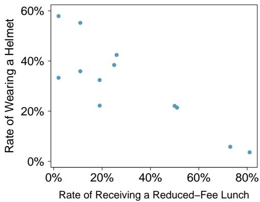
Problem 10: Helmets and lunches. The scatterplot shows the relationship between socioeconomic status measured as the percentage of children in a neighborhood receiving reduced-fee lunches at school (lunch) and the percentage of bike riders in the neighborhood wearing helmets (helmet). The average percentage of children receiving reduced-fee lunches is \(30.8\%\) with a standard deviation of \(26.7\%\), and the average percentage of bike riders wearing helmets is \(38.8\%\) with a standard deviation of \(16.9\%\).
(a) If the \(R^2\) for the least-squares regression line for these data is \(72\%\), what is the correlation between lunch and helmet?
(b) Calculate the slope and intercept for the least-squares regression line for these data.
(c) Interpret the intercept of the least-squares regression line in the context of the application.
(d) Interpret the slope of the least-squares regression line in the context of the application.
(e) What would the value of the residual be for a neighborhood where \(40\%\) of the children receive reduced-fee lunches and \(40\%\) of the bike riders wear helmets? Interpret the meaning of this residual in the context of the application.
Problem 8.42 Solution
Step 1 — Correlation from \(R^2\) (a): $$r = \pm\sqrt{0.72} = \pm 0.849.$$ Higher reduced-lunch percentages are expected to correspond to lower helmet-wearing percentages (a neighborhood-SES pattern), so the slope is negative and \(r \approx -0.849\).
Step 2 — Slope of the least-squares line (b): $$b = r \cdot \frac{s_y}{s_x} = -0.849 \cdot \frac{16.9}{26.7} \approx -0.537.$$
Step 3 — Intercept: The regression line passes through \((\bar{x}, \bar{y}) = (30.8, 38.8)\): $$a = \bar{y} - b \bar{x} = 38.8 - (-0.537)(30.8) = 38.8 + 16.54 \approx 55.3.$$ So $$\widehat{\text{helmet}} = 55.3 - 0.537 \times \text{lunch}.$$
Step 4 — Interpret the intercept (c): At a hypothetical neighborhood where \(0\%\) of children receive reduced-fee lunches, the predicted helmet-wearing rate is about \(55.3\%\). Interpret cautiously — this may extrapolate beyond the data.
Step 5 — Interpret the slope (d): For each additional 1 percentage point of children receiving reduced-fee lunches, the predicted percentage of bike riders wearing helmets decreases by about \(0.54\) percentage points.
Step 6 — Residual at (40%, 40%) (e): $$\widehat{\text{helmet}} = 55.3 - 0.537 \times 40 = 55.3 - 21.48 = 33.82.$$ Residual \(= y - \hat{y} = 40 - 33.82 = 6.18\). The actual helmet rate is about \(6.2\) percentage points higher than the model predicts — the neighborhood does better than expected.
Answer: (a) \(r \approx -0.85\). (b) \(b \approx -0.54\), \(a \approx 55.3\). (c)–(d) See steps 4–5. (e) Residual \(\approx +6.2\) percentage points.
Problem 11: Match the correlation, Part III. Match each correlation to the corresponding scatterplot.
(a) \(r = -0.72\)
(b) \(r = 0.07\)
(c) \(r = 0.86\)
(d) \(r = 0.99\)
(1)
(2)
(3)
(4)
Problem 8.43 Solution
Step 1 — Rank the correlations by strength: Order by \(|r|\): \(|0.99| > |0.86| > |{-0.72}| > |0.07|\).
Step 2 — Match strongest positive (\(r = 0.99\)): The plot that looks like an almost perfect straight line with positive slope and very little scatter — very tight cluster around a rising line.
Step 3 — Match strong positive (\(r = 0.86\)): Still clearly positive and linear but with visibly more scatter than the \(0.99\) plot.
Step 4 — Match strong negative (\(r = -0.72\)): A plot with a clearly decreasing linear trend and moderate scatter.
Step 5 — Match near-zero (\(r = 0.07\)): A plot with essentially no visible trend — a near-circular cloud of points.
Answer: Strongest-to-weakest by |r|: (d) \(0.99\), (c) \(0.86\), (a) \(-0.72\), (b) \(0.07\). The unique pairing is the tightest positive line \(\to 0.99\), the noisier positive line \(\to 0.86\), the decreasing line \(\to -0.72\), and the patternless cloud \(\to 0.07\).
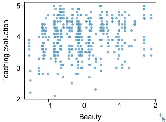
Problem 12: Rate my professor. Many college courses conclude by giving students the opportunity to evaluate the course and the instructor anonymously. However, the use of these student evaluations as an indicator of course quality and teaching effectiveness is often criticized because these measures may reflect the influence of non-teaching-related characteristics, such as the physical appearance of the instructor. Researchers at University of Texas, Austin collected data on teaching evaluation score (higher score means better) and standardized beauty score (a score of 0 means average, negative score means below average, and a positive score means above average) for a sample of 463 professors. The scatterplot below shows the relationship between these variables, and regression output is provided for predicting teaching evaluation score from beauty score.
| Estimate | Std. Error | t value | Pr(>|t|) | |
| (Intercept) | 4.010 | 0.0255 | 157.21 | 0.0000 |
| beauty | □ | 0.0322 | 4.13 | 0.0000 |
(a) Given that the average standardized beauty score is \(-0.0883\) and average teaching evaluation score is \(3.9983\), calculate the slope. Alternatively, the slope may be computed using just the information provided in the model summary table.
(b) Do these data provide convincing evidence that the slope of the relationship between teaching evaluation and beauty is positive? Explain your reasoning.
(c) List the conditions required for linear regression and check if each one is satisfied for this model based on the following diagnostic plots.
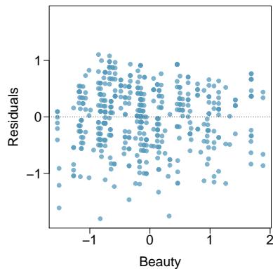
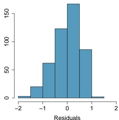
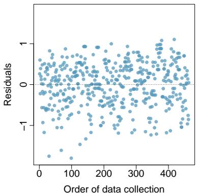
Problem 8.44 Solution
Step 1 — Calculate the slope (a):
The regression line must pass through \((\bar{x}, \bar{y}) = (-0.0883,\ 3.9983)\), so
$$\bar{y} = a + b \bar{x} \;\Longrightarrow\; 3.9983 = 4.010 + b(-0.0883).$$
Solve:
$$b = \frac{3.9983 - 4.010}{-0.0883} = \frac{-0.0117}{-0.0883} \approx 0.133.$$
(Equivalently, the t value of \(4.13\) with \(SE = 0.0322\) gives \(b = 4.13 \times 0.0322 \approx 0.133\), confirming the estimate.)
Step 2 — Positive slope test (b): Hypotheses: \(H_0: \beta = 0\) vs. \(H_A: \beta > 0\). The reported two-sided p-value is \(0.0000\) and the observed slope is positive, so the one-sided p-value is essentially \(0\). We reject \(H_0\): yes, there is convincing evidence that higher beauty scores are associated with higher teaching evaluation scores.
Step 3 — Check conditions (c): Using the diagnostic plots: - Linearity: Residual plot should show no ∪-shape or curved pattern. - Constant variability: Residuals should have roughly the same spread across \(x\). - Nearly normal residuals: \(n = 463 \ge 30\), so this condition is automatically satisfied by the large sample size. - Independence: Assume data come from a reasonably representative sample of professors.
If the residual/Q-Q plots look like random scatter with constant spread and roughly normal residuals, all four conditions are met. The large \(n\) in particular makes the inference robust.
Answer: (a) \(b \approx 0.133\). (b) Reject \(H_0\); evidence of a positive linear relationship. (c) All four conditions are reasonably satisfied, assuming diagnostic plots show no strong patterns.
Problem 13: Trees. The scatterplots below show the relationship between height, diameter, and volume of timber in 31 felled black cherry trees. The diameter of the tree is measured 4.5 feet above the ground.
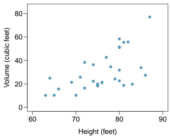
(a) Describe the relationship between volume and height of these trees.
(b) Describe the relationship between volume and diameter of these trees.
(c) Suppose you have height and diameter measurements for another black cherry tree. Which of these variables would be preferable to use to predict the volume of timber in this tree using a simple linear regression model? Explain your reasoning.
Problem 8.45 Solution
Step 1 — Volume vs. height (a): The scatterplot shows a positive association between volume and height: taller trees tend to contain more timber. The relationship looks roughly linear but with substantial scatter — some tall trees have moderate volume and vice versa.
Step 2 — Volume vs. diameter (b): The scatterplot shows a strong, positive, and clearly curved association: volume increases sharply with diameter. Because volume scales roughly with \(\text{diameter}^2\) (think of a cylinder: \(V \propto d^2 h\)), the relationship is not linear — it bends upward.
Step 3 — Which predictor to use (c): Diameter is the better predictor of timber volume because the diameter-volume relationship is much stronger than the height-volume relationship (higher \(R^2\)). However, the curvature in the diameter-volume plot means a simple linear regression may not be ideal; a transformation (e.g., predicting volume from \(\text{diameter}^2\) or using \(\log(\text{volume})\) vs. \(\log(\text{diameter})\)) would usually fit much better. If we insist on a single linear predictor, diameter still wins, but the residual plot should be checked to justify the linearity assumption.
Answer: (a) Moderate positive, roughly linear association. (b) Strong positive but clearly curved association. (c) Diameter — stronger relationship — though a transformation would improve the linearity.